EPPS 6323: Lab02

R Programming Basic Commands

(Adapted from ISLR Chapter 3 Lab: Introduction to R)

Indexing Data using []

A=matrix(1:16,4,4)
A

     [,1] [,2] [,3] [,4]
[1,]    1    5    9   13
[2,]    2    6   10   14
[3,]    3    7   11   15
[4,]    4    8   12   16

A[2,3]

[1] 10

A[c(1,3),c(2,4)]

     [,1] [,2]
[1,]    5   13
[2,]    7   15

A[1:3,2:4]

     [,1] [,2] [,3]
[1,]    5    9   13
[2,]    6   10   14
[3,]    7   11   15

A[1:2,]

     [,1] [,2] [,3] [,4]
[1,]    1    5    9   13
[2,]    2    6   10   14

A[,1:2]

     [,1] [,2]
[1,]    1    5
[2,]    2    6
[3,]    3    7
[4,]    4    8

A[1,]

[1]  1  5  9 13

A[-c(1,3),]

     [,1] [,2] [,3] [,4]
[1,]    2    6   10   14
[2,]    4    8   12   16

A[-c(1,3),-c(1,3,4)]

[1] 6 8

dim(A)

[1] 4 4

Loading Data from GitHub

Auto=read.table("https://raw.githubusercontent.com/karlho/knowledgemining/gh-pages/data/Auto.data")
# fix(Auto) # Starting the X11 R data editor
Auto=read.table("https://raw.githubusercontent.com/karlho/knowledgemining/gh-pages/data/Auto.data",header=T,na.strings="?")
# fix(Auto)
Auto=read.csv("https://raw.githubusercontent.com/karlho/knowledgemining/gh-pages/data/Auto.csv",header=T,na.strings="?")
# fix(Auto)
dim(Auto)

[1] 397   9

Auto[1:4,]

  mpg cylinders displacement horsepower weight acceleration year origin
1  18         8          307        130   3504         12.0   70      1
2  15         8          350        165   3693         11.5   70      1
3  18         8          318        150   3436         11.0   70      1
4  16         8          304        150   3433         12.0   70      1
                       name
1 chevrolet chevelle malibu
2         buick skylark 320
3        plymouth satellite
4             amc rebel sst

Auto=na.omit(Auto)
dim(Auto)

[1] 392   9

names(Auto)

[1] "mpg"          "cylinders"    "displacement" "horsepower"   "weight"      
[6] "acceleration" "year"         "origin"       "name"        

Load data from ISLR website

Auto=read.table("https://www.statlearning.com/s/Auto.data",header=T,na.strings="?")
dim(Auto)

[1] 397   9

Additional Graphical and Numerical Summaries

# plot(cylinders, mpg)
plot(Auto$cylinders, Auto$mpg)

attach(Auto)
plot(cylinders, mpg)

cylinders=as.factor(cylinders)
plot(cylinders, mpg)

plot(cylinders, mpg, col="red")

plot(cylinders, mpg, col="red", varwidth=T)

plot(cylinders, mpg, col="red", varwidth=T,horizontal=T)

plot(cylinders, mpg, col="red", varwidth=T, xlab="cylinders", ylab="MPG")

hist(mpg)

hist(mpg,col=2)

hist(mpg,col=2,breaks=15)

#pairs(Auto)
pairs(~ mpg + displacement + horsepower + weight + acceleration, Auto)

plot(horsepower,mpg)

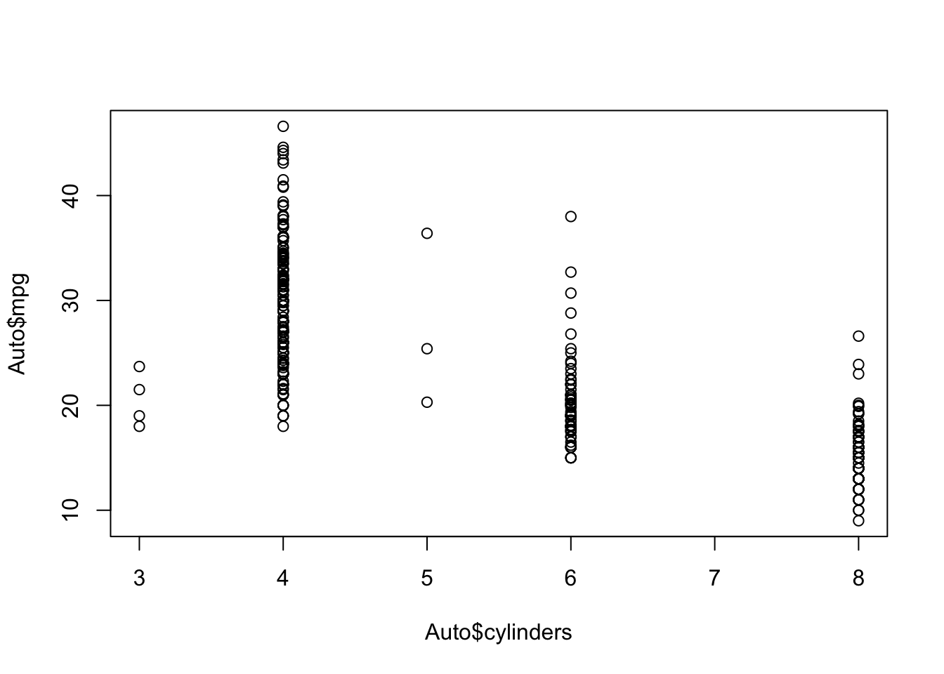
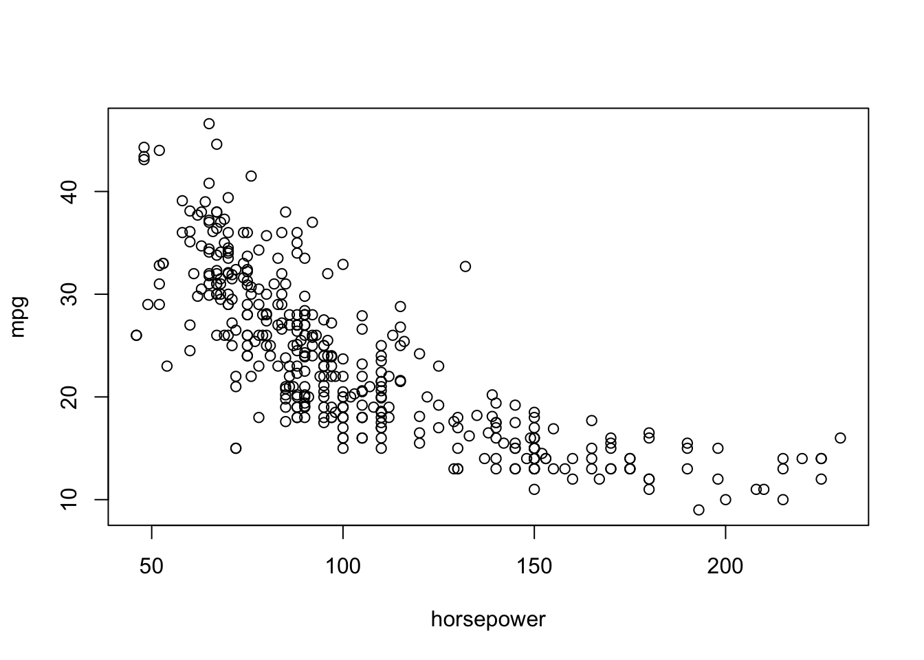
# identify(horsepower,mpg,name) # Interactive: point and click the dot to identify cases
summary(Auto)

      mpg          cylinders      displacement     horsepower        weight    
 Min.   : 9.00   Min.   :3.000   Min.   : 68.0   Min.   : 46.0   Min.   :1613  
 1st Qu.:17.50   1st Qu.:4.000   1st Qu.:104.0   1st Qu.: 75.0   1st Qu.:2223  
 Median :23.00   Median :4.000   Median :146.0   Median : 93.5   Median :2800  
 Mean   :23.52   Mean   :5.458   Mean   :193.5   Mean   :104.5   Mean   :2970  
 3rd Qu.:29.00   3rd Qu.:8.000   3rd Qu.:262.0   3rd Qu.:126.0   3rd Qu.:3609  
 Max.   :46.60   Max.   :8.000   Max.   :455.0   Max.   :230.0   Max.   :5140  
                                                 NA's   :5                     
  acceleration        year           origin          name          
 Min.   : 8.00   Min.   :70.00   Min.   :1.000   Length:397        
 1st Qu.:13.80   1st Qu.:73.00   1st Qu.:1.000   Class :character  
 Median :15.50   Median :76.00   Median :1.000   Mode  :character  
 Mean   :15.56   Mean   :75.99   Mean   :1.574                     
 3rd Qu.:17.10   3rd Qu.:79.00   3rd Qu.:2.000                     
 Max.   :24.80   Max.   :82.00   Max.   :3.000                     
                                                                   

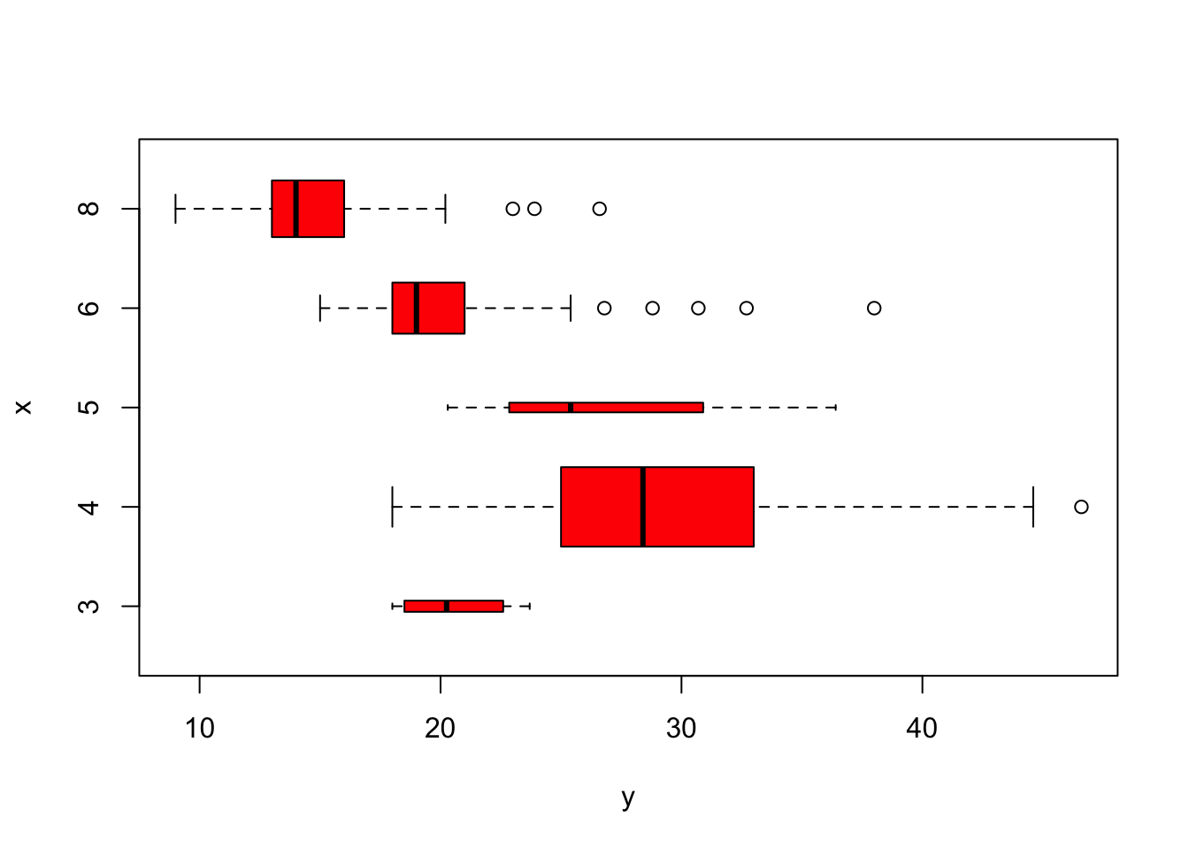
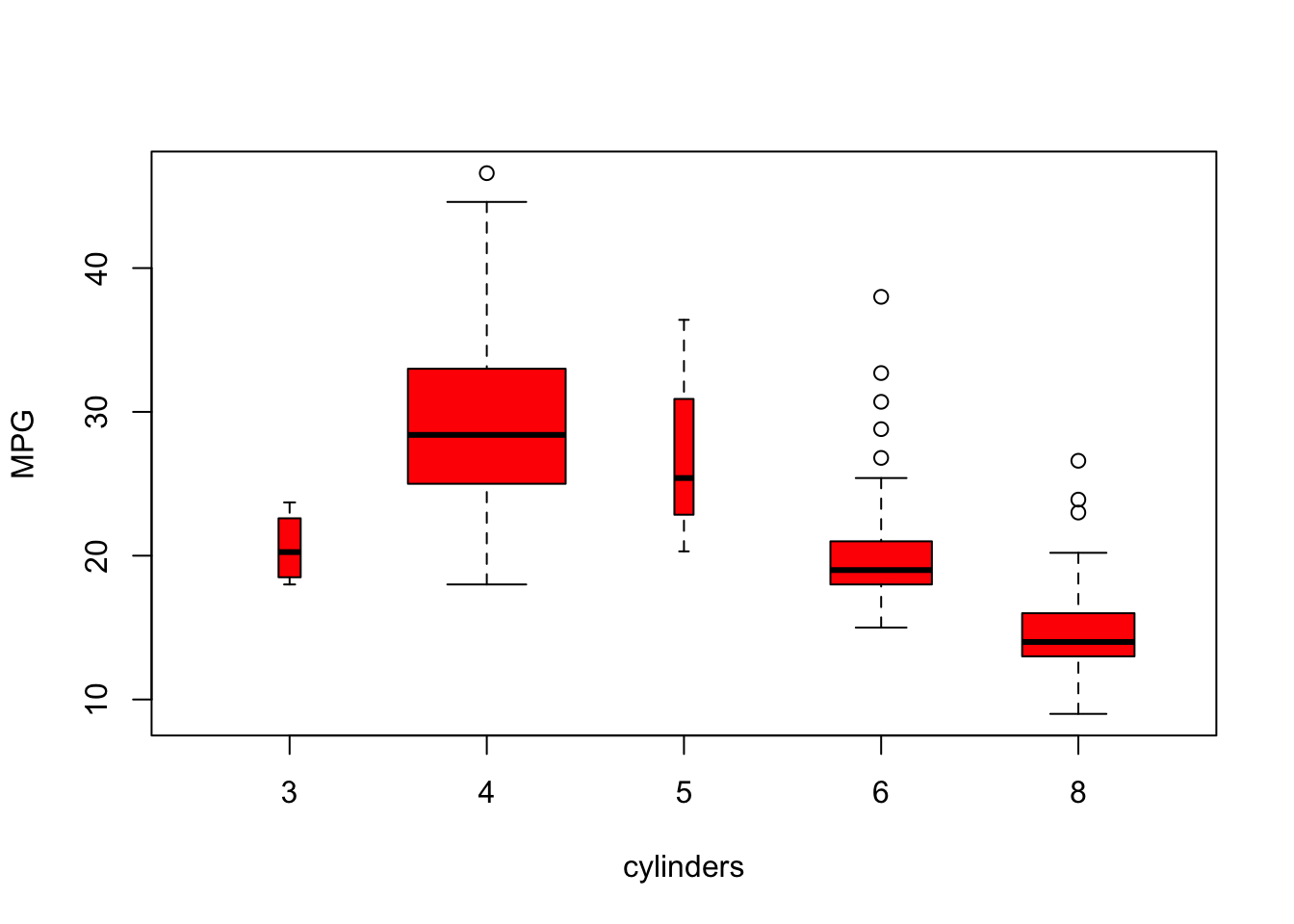
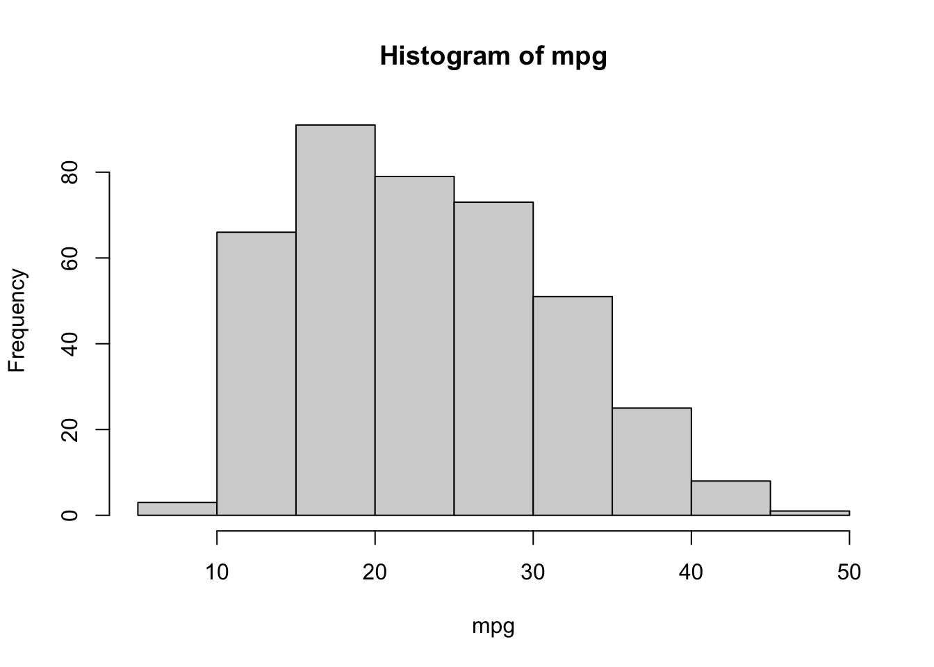
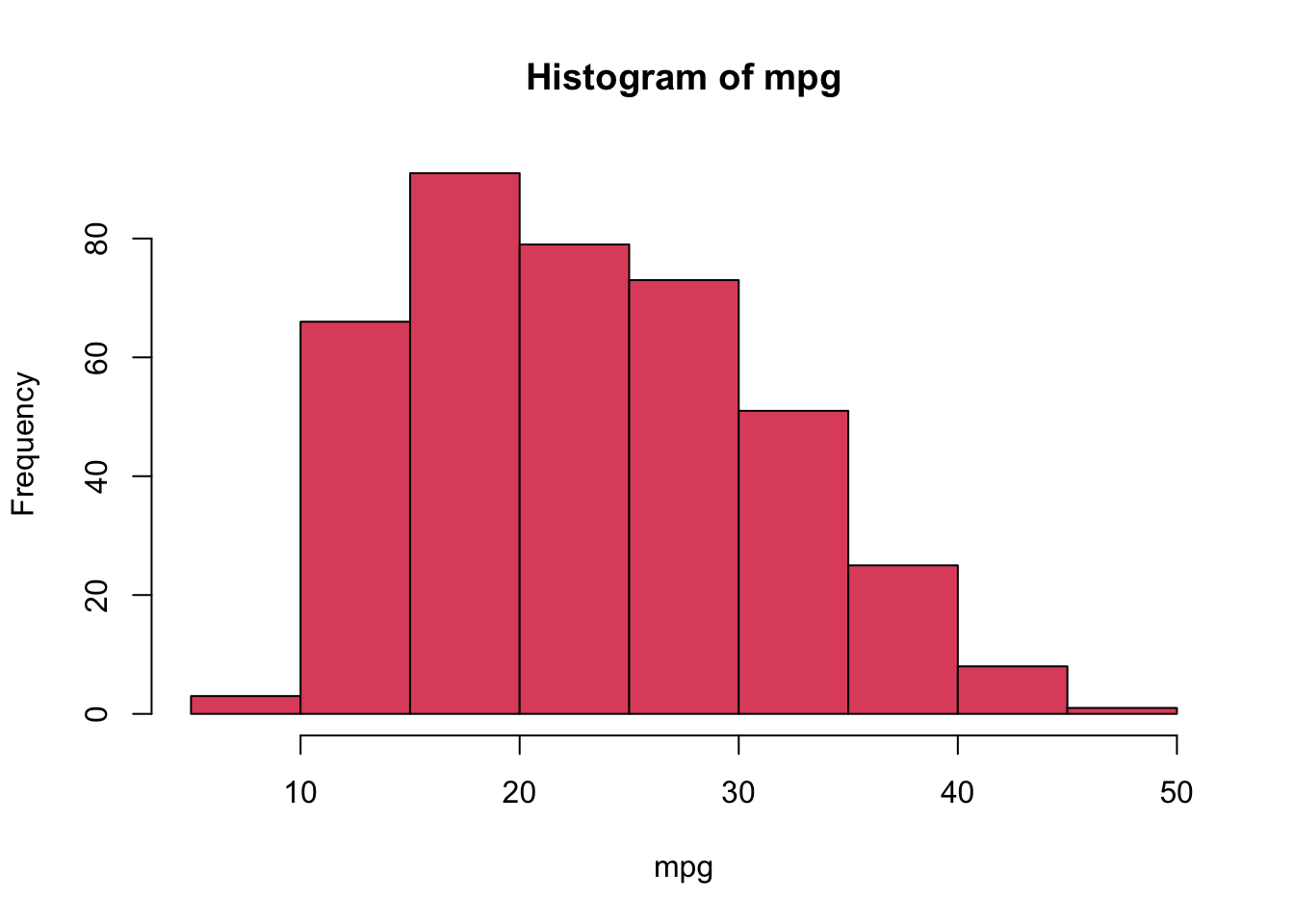
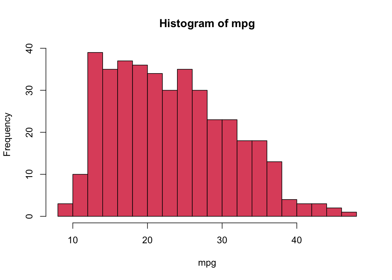
summary(mpg)

   Min. 1st Qu.  Median    Mean 3rd Qu.    Max. 
   9.00   17.50   23.00   23.52   29.00   46.60 

Linear Regression

ptbu=c("MASS","ISLR")
install.packages(ptbu, repos='http://cran.us.r-project.org')

The downloaded binary packages are in
    /var/folders/fg/l9nwkw5954b_7xv794xmt5_40000gn/T//Rtmpzv3uXL/downloaded_packages

lapply(ptbu, require, character.only = TRUE)

Loading required package: MASS

Loading required package: ISLR

Attaching package: 'ISLR'

The following object is masked _by_ '.GlobalEnv':

    Auto

[[1]]
[1] TRUE

[[2]]
[1] TRUE

library(MASS)
library(ISLR)

# Simple Linear Regression

# fix(Boston)
names(Boston)

 [1] "crim"    "zn"      "indus"   "chas"    "nox"     "rm"      "age"    
 [8] "dis"     "rad"     "tax"     "ptratio" "black"   "lstat"   "medv"   

# lm.fit=lm(medv~lstat)
attach(Boston)
lm.fit=lm(medv~lstat,data=Boston)
attach(Boston)

The following objects are masked from Boston (pos = 3):

    age, black, chas, crim, dis, indus, lstat, medv, nox, ptratio, rad,
    rm, tax, zn

lm.fit=lm(medv~lstat)
lm.fit

Call:
lm(formula = medv ~ lstat)

Coefficients:
(Intercept)        lstat  
      34.55        -0.95  

summary(lm.fit)

Call:
lm(formula = medv ~ lstat)

Residuals:
    Min      1Q  Median      3Q     Max 
-15.168  -3.990  -1.318   2.034  24.500 

Coefficients:
            Estimate Std. Error t value Pr(>|t|)    
(Intercept) 34.55384    0.56263   61.41   <2e-16 ***
lstat       -0.95005    0.03873  -24.53   <2e-16 ***
---
Signif. codes:  0 '***' 0.001 '**' 0.01 '*' 0.05 '.' 0.1 ' ' 1

Residual standard error: 6.216 on 504 degrees of freedom
Multiple R-squared:  0.5441,    Adjusted R-squared:  0.5432 
F-statistic: 601.6 on 1 and 504 DF,  p-value: < 2.2e-16

names(lm.fit)

 [1] "coefficients"  "residuals"     "effects"       "rank"         
 [5] "fitted.values" "assign"        "qr"            "df.residual"  
 [9] "xlevels"       "call"          "terms"         "model"        

coef(lm.fit)

(Intercept)       lstat 
 34.5538409  -0.9500494 

confint(lm.fit)

                2.5 %     97.5 %
(Intercept) 33.448457 35.6592247
lstat       -1.026148 -0.8739505

predict(lm.fit,data.frame(lstat=(c(5,10,15))), interval="confidence")

       fit      lwr      upr
1 29.80359 29.00741 30.59978
2 25.05335 24.47413 25.63256
3 20.30310 19.73159 20.87461

predict(lm.fit,data.frame(lstat=(c(5,10,15))), interval="prediction")

       fit       lwr      upr
1 29.80359 17.565675 42.04151
2 25.05335 12.827626 37.27907
3 20.30310  8.077742 32.52846

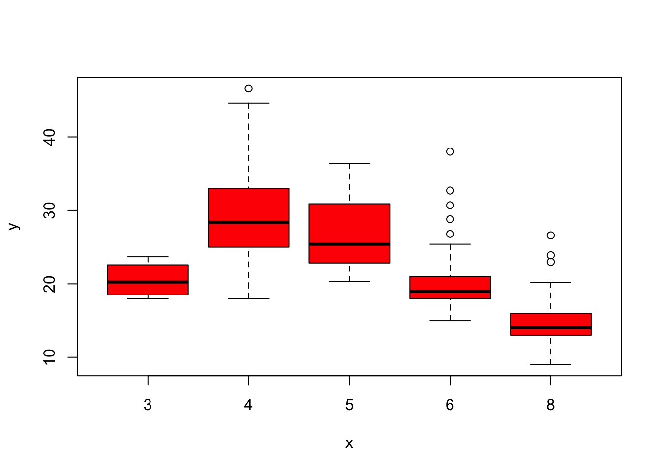
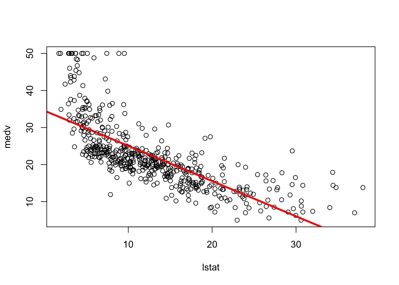
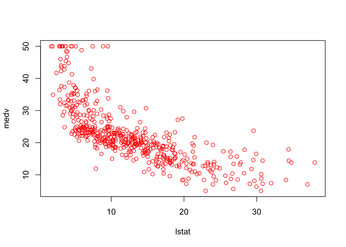
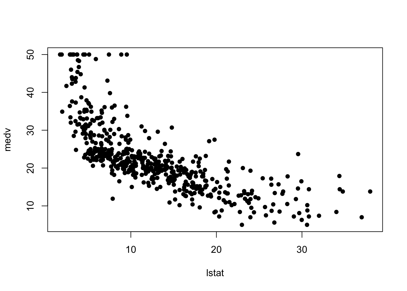
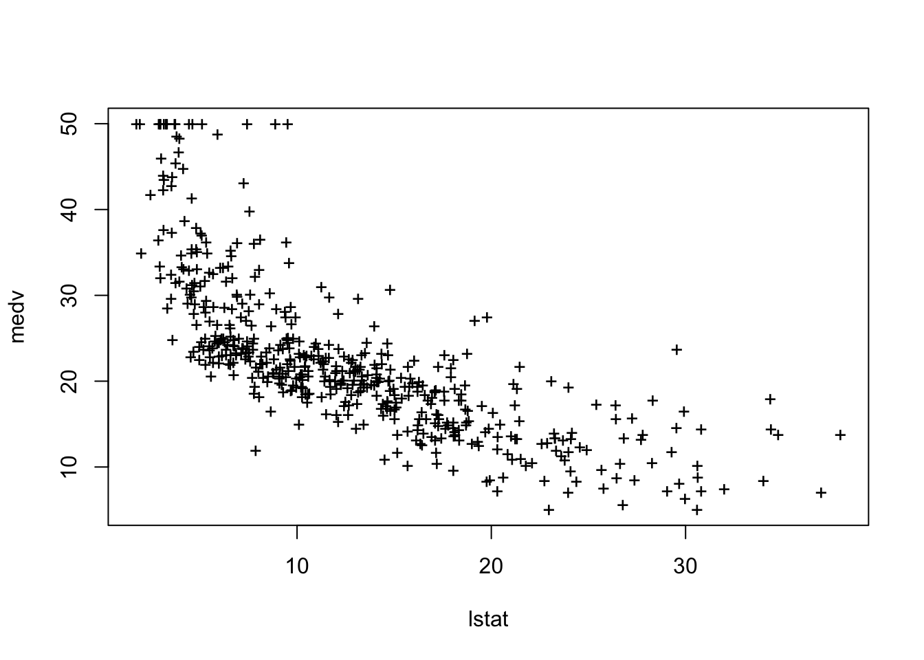
# What is the differnce between "conference" and "prediction" difference?

plot(lstat,medv)
abline(lm.fit)
abline(lm.fit,lwd=3)
abline(lm.fit,lwd=3,col="red")

plot(lstat,medv,col="red")

plot(lstat,medv,pch=16)

plot(lstat,medv,pch="+")

plot(1:20,1:20,pch=1:20)

par(mfrow=c(2,2))
plot(lm.fit)

plot(predict(lm.fit), residuals(lm.fit))
plot(predict(lm.fit), rstudent(lm.fit))
plot(hatvalues(lm.fit))
which.max(hatvalues(lm.fit))

375 
375 

Multiple Linear Regression

lm.fit=lm(medv~lstat+age,data=Boston)
summary(lm.fit)

Call:
lm(formula = medv ~ lstat + age, data = Boston)

Residuals:
    Min      1Q  Median      3Q     Max 
-15.981  -3.978  -1.283   1.968  23.158 

Coefficients:
            Estimate Std. Error t value Pr(>|t|)    
(Intercept) 33.22276    0.73085  45.458  < 2e-16 ***
lstat       -1.03207    0.04819 -21.416  < 2e-16 ***
age          0.03454    0.01223   2.826  0.00491 ** 
---
Signif. codes:  0 '***' 0.001 '**' 0.01 '*' 0.05 '.' 0.1 ' ' 1

Residual standard error: 6.173 on 503 degrees of freedom
Multiple R-squared:  0.5513,    Adjusted R-squared:  0.5495 
F-statistic:   309 on 2 and 503 DF,  p-value: < 2.2e-16

lm.fit=lm(medv~.,data=Boston)
summary(lm.fit)

Call:
lm(formula = medv ~ ., data = Boston)

Residuals:
    Min      1Q  Median      3Q     Max 
-15.595  -2.730  -0.518   1.777  26.199 

Coefficients:
              Estimate Std. Error t value Pr(>|t|)    
(Intercept)  3.646e+01  5.103e+00   7.144 3.28e-12 ***
crim        -1.080e-01  3.286e-02  -3.287 0.001087 ** 
zn           4.642e-02  1.373e-02   3.382 0.000778 ***
indus        2.056e-02  6.150e-02   0.334 0.738288    
chas         2.687e+00  8.616e-01   3.118 0.001925 ** 
nox         -1.777e+01  3.820e+00  -4.651 4.25e-06 ***
rm           3.810e+00  4.179e-01   9.116  < 2e-16 ***
age          6.922e-04  1.321e-02   0.052 0.958229    
dis         -1.476e+00  1.995e-01  -7.398 6.01e-13 ***
rad          3.060e-01  6.635e-02   4.613 5.07e-06 ***
tax         -1.233e-02  3.760e-03  -3.280 0.001112 ** 
ptratio     -9.527e-01  1.308e-01  -7.283 1.31e-12 ***
black        9.312e-03  2.686e-03   3.467 0.000573 ***
lstat       -5.248e-01  5.072e-02 -10.347  < 2e-16 ***
---
Signif. codes:  0 '***' 0.001 '**' 0.01 '*' 0.05 '.' 0.1 ' ' 1

Residual standard error: 4.745 on 492 degrees of freedom
Multiple R-squared:  0.7406,    Adjusted R-squared:  0.7338 
F-statistic: 108.1 on 13 and 492 DF,  p-value: < 2.2e-16

library(car)

Loading required package: carData

vif(lm.fit)

    crim       zn    indus     chas      nox       rm      age      dis 
1.792192 2.298758 3.991596 1.073995 4.393720 1.933744 3.100826 3.955945 
     rad      tax  ptratio    black    lstat 
7.484496 9.008554 1.799084 1.348521 2.941491 

lm.fit1=lm(medv~.-age,data=Boston)
summary(lm.fit1)

Call:
lm(formula = medv ~ . - age, data = Boston)

Residuals:
     Min       1Q   Median       3Q      Max 
-15.6054  -2.7313  -0.5188   1.7601  26.2243 

Coefficients:
              Estimate Std. Error t value Pr(>|t|)    
(Intercept)  36.436927   5.080119   7.172 2.72e-12 ***
crim         -0.108006   0.032832  -3.290 0.001075 ** 
zn            0.046334   0.013613   3.404 0.000719 ***
indus         0.020562   0.061433   0.335 0.737989    
chas          2.689026   0.859598   3.128 0.001863 ** 
nox         -17.713540   3.679308  -4.814 1.97e-06 ***
rm            3.814394   0.408480   9.338  < 2e-16 ***
dis          -1.478612   0.190611  -7.757 5.03e-14 ***
rad           0.305786   0.066089   4.627 4.75e-06 ***
tax          -0.012329   0.003755  -3.283 0.001099 ** 
ptratio      -0.952211   0.130294  -7.308 1.10e-12 ***
black         0.009321   0.002678   3.481 0.000544 ***
lstat        -0.523852   0.047625 -10.999  < 2e-16 ***
---
Signif. codes:  0 '***' 0.001 '**' 0.01 '*' 0.05 '.' 0.1 ' ' 1

Residual standard error: 4.74 on 493 degrees of freedom
Multiple R-squared:  0.7406,    Adjusted R-squared:  0.7343 
F-statistic: 117.3 on 12 and 493 DF,  p-value: < 2.2e-16

lm.fit1=update(lm.fit, ~.-age)

Non-linear Transformations of the Predictors

lm.fit2=lm(medv~lstat+I(lstat^2))
summary(lm.fit2)

Call:
lm(formula = medv ~ lstat + I(lstat^2))

Residuals:
     Min       1Q   Median       3Q      Max 
-15.2834  -3.8313  -0.5295   2.3095  25.4148 

Coefficients:
             Estimate Std. Error t value Pr(>|t|)    
(Intercept) 42.862007   0.872084   49.15   <2e-16 ***
lstat       -2.332821   0.123803  -18.84   <2e-16 ***
I(lstat^2)   0.043547   0.003745   11.63   <2e-16 ***
---
Signif. codes:  0 '***' 0.001 '**' 0.01 '*' 0.05 '.' 0.1 ' ' 1

Residual standard error: 5.524 on 503 degrees of freedom
Multiple R-squared:  0.6407,    Adjusted R-squared:  0.6393 
F-statistic: 448.5 on 2 and 503 DF,  p-value: < 2.2e-16

lm.fit=lm(medv~lstat)
anova(lm.fit,lm.fit2)

Analysis of Variance Table

Model 1: medv ~ lstat
Model 2: medv ~ lstat + I(lstat^2)
  Res.Df   RSS Df Sum of Sq     F    Pr(>F)    
1    504 19472                                 
2    503 15347  1    4125.1 135.2 < 2.2e-16 ***
---
Signif. codes:  0 '***' 0.001 '**' 0.01 '*' 0.05 '.' 0.1 ' ' 1

par(mfrow=c(2,2))
plot(lm.fit2)

lm.fit5=lm(medv~poly(lstat,5))
summary(lm.fit5)

Call:
lm(formula = medv ~ poly(lstat, 5))

Residuals:
     Min       1Q   Median       3Q      Max 
-13.5433  -3.1039  -0.7052   2.0844  27.1153 

Coefficients:
                 Estimate Std. Error t value Pr(>|t|)    
(Intercept)       22.5328     0.2318  97.197  < 2e-16 ***
poly(lstat, 5)1 -152.4595     5.2148 -29.236  < 2e-16 ***
poly(lstat, 5)2   64.2272     5.2148  12.316  < 2e-16 ***
poly(lstat, 5)3  -27.0511     5.2148  -5.187 3.10e-07 ***
poly(lstat, 5)4   25.4517     5.2148   4.881 1.42e-06 ***
poly(lstat, 5)5  -19.2524     5.2148  -3.692 0.000247 ***
---
Signif. codes:  0 '***' 0.001 '**' 0.01 '*' 0.05 '.' 0.1 ' ' 1

Residual standard error: 5.215 on 500 degrees of freedom
Multiple R-squared:  0.6817,    Adjusted R-squared:  0.6785 
F-statistic: 214.2 on 5 and 500 DF,  p-value: < 2.2e-16

summary(lm(medv~log(rm),data=Boston))

Call:
lm(formula = medv ~ log(rm), data = Boston)

Residuals:
    Min      1Q  Median      3Q     Max 
-19.487  -2.875  -0.104   2.837  39.816 

Coefficients:
            Estimate Std. Error t value Pr(>|t|)    
(Intercept)  -76.488      5.028  -15.21   <2e-16 ***
log(rm)       54.055      2.739   19.73   <2e-16 ***
---
Signif. codes:  0 '***' 0.001 '**' 0.01 '*' 0.05 '.' 0.1 ' ' 1

Residual standard error: 6.915 on 504 degrees of freedom
Multiple R-squared:  0.4358,    Adjusted R-squared:  0.4347 
F-statistic: 389.3 on 1 and 504 DF,  p-value: < 2.2e-16

Qualitative Predictors

# fix(Carseats)
names(Carseats)

 [1] "Sales"       "CompPrice"   "Income"      "Advertising" "Population" 
 [6] "Price"       "ShelveLoc"   "Age"         "Education"   "Urban"      
[11] "US"         

lm.fit=lm(Sales~.+Income:Advertising+Price:Age,data=Carseats)
summary(lm.fit)

Call:
lm(formula = Sales ~ . + Income:Advertising + Price:Age, data = Carseats)

Residuals:
    Min      1Q  Median      3Q     Max 
-2.9208 -0.7503  0.0177  0.6754  3.3413 

Coefficients:
                     Estimate Std. Error t value Pr(>|t|)    
(Intercept)         6.5755654  1.0087470   6.519 2.22e-10 ***
CompPrice           0.0929371  0.0041183  22.567  < 2e-16 ***
Income              0.0108940  0.0026044   4.183 3.57e-05 ***
Advertising         0.0702462  0.0226091   3.107 0.002030 ** 
Population          0.0001592  0.0003679   0.433 0.665330    
Price              -0.1008064  0.0074399 -13.549  < 2e-16 ***
ShelveLocGood       4.8486762  0.1528378  31.724  < 2e-16 ***
ShelveLocMedium     1.9532620  0.1257682  15.531  < 2e-16 ***
Age                -0.0579466  0.0159506  -3.633 0.000318 ***
Education          -0.0208525  0.0196131  -1.063 0.288361    
UrbanYes            0.1401597  0.1124019   1.247 0.213171    
USYes              -0.1575571  0.1489234  -1.058 0.290729    
Income:Advertising  0.0007510  0.0002784   2.698 0.007290 ** 
Price:Age           0.0001068  0.0001333   0.801 0.423812    
---
Signif. codes:  0 '***' 0.001 '**' 0.01 '*' 0.05 '.' 0.1 ' ' 1

Residual standard error: 1.011 on 386 degrees of freedom
Multiple R-squared:  0.8761,    Adjusted R-squared:  0.8719 
F-statistic:   210 on 13 and 386 DF,  p-value: < 2.2e-16

attach(Carseats)
contrasts(ShelveLoc)

       Good Medium
Bad       0      0
Good      1      0
Medium    0      1

Interaction Terms (including interaction and single effects)

summary(lm(medv~lstat*age,data=Boston))

Call:
lm(formula = medv ~ lstat * age, data = Boston)

Residuals:
    Min      1Q  Median      3Q     Max 
-15.806  -4.045  -1.333   2.085  27.552 

Coefficients:
              Estimate Std. Error t value Pr(>|t|)    
(Intercept) 36.0885359  1.4698355  24.553  < 2e-16 ***
lstat       -1.3921168  0.1674555  -8.313 8.78e-16 ***
age         -0.0007209  0.0198792  -0.036   0.9711    
lstat:age    0.0041560  0.0018518   2.244   0.0252 *  
---
Signif. codes:  0 '***' 0.001 '**' 0.01 '*' 0.05 '.' 0.1 ' ' 1

Residual standard error: 6.149 on 502 degrees of freedom
Multiple R-squared:  0.5557,    Adjusted R-squared:  0.5531 
F-statistic: 209.3 on 3 and 502 DF,  p-value: < 2.2e-16