# Prediction interval uses sample mean and takes into account the variability of the estimators for μ and σ.# Therefore, the interval will be wider.### Multiple linear regressionfit2=lm(medv~lstat+age,data=Boston)summary(fit2)
Call:
lm(formula = medv ~ lstat + age, data = Boston)

Residuals:
    Min      1Q  Median      3Q     Max
-15.981  -3.978  -1.283   1.968  23.158

Coefficients:
            Estimate Std. Error t value Pr(>|t|)
(Intercept) 33.22276    0.73085  45.458  < 2e-16 ***
lstat       -1.03207    0.04819 -21.416  < 2e-16 ***
age          0.03454    0.01223   2.826  0.00491 **
---
Signif. codes:  0 '***' 0.001 '**' 0.01 '*' 0.05 '.' 0.1 ' ' 1

Residual standard error: 6.173 on 503 degrees of freedom
Multiple R-squared:  0.5513,    Adjusted R-squared:  0.5495
F-statistic:   309 on 2 and 503 DF,  p-value: < 2.2e-16
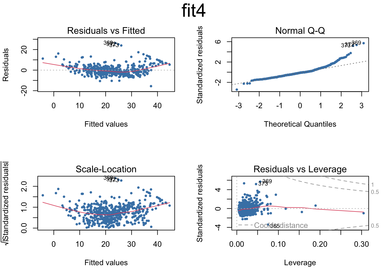
# Set the next plot configurationpar(mfrow=c(2,2), main="fit4")
Warning in par(mfrow = c(2, 2), main = "fit4"): "main" is not a graphical
parameter
plot(fit4,pch=20, cex=.8, col="steelblue")mtext("fit4", side =3, line =-2, cex =2, outer =TRUE)
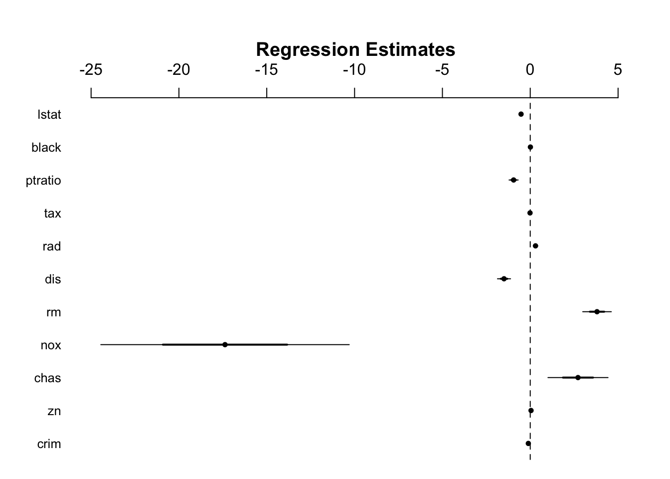
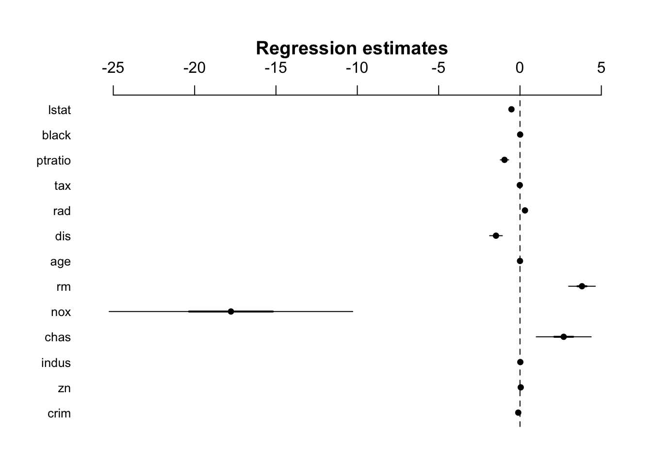
# Uses coefplot to plot coefficients. Note the line at 0.par(mfrow=c(1,1))arm::coefplot(fit4)
### Nonlinear terms and Interactionsfit5=lm(medv~lstat*age,Boston) # include both variables and the interaction term x1:x2summary(fit5)
Call:
lm(formula = medv ~ lstat * age, data = Boston)

Residuals:
    Min      1Q  Median      3Q     Max
-15.806  -4.045  -1.333   2.085  27.552

Coefficients:
              Estimate Std. Error t value Pr(>|t|)
(Intercept) 36.0885359  1.4698355  24.553  < 2e-16 ***
lstat       -1.3921168  0.1674555  -8.313 8.78e-16 ***
age         -0.0007209  0.0198792  -0.036   0.9711
lstat:age    0.0041560  0.0018518   2.244   0.0252 *
---
Signif. codes:  0 '***' 0.001 '**' 0.01 '*' 0.05 '.' 0.1 ' ' 1

Residual standard error: 6.149 on 502 degrees of freedom
Multiple R-squared:  0.5557,    Adjusted R-squared:  0.5531
F-statistic: 209.3 on 3 and 502 DF,  p-value: < 2.2e-16
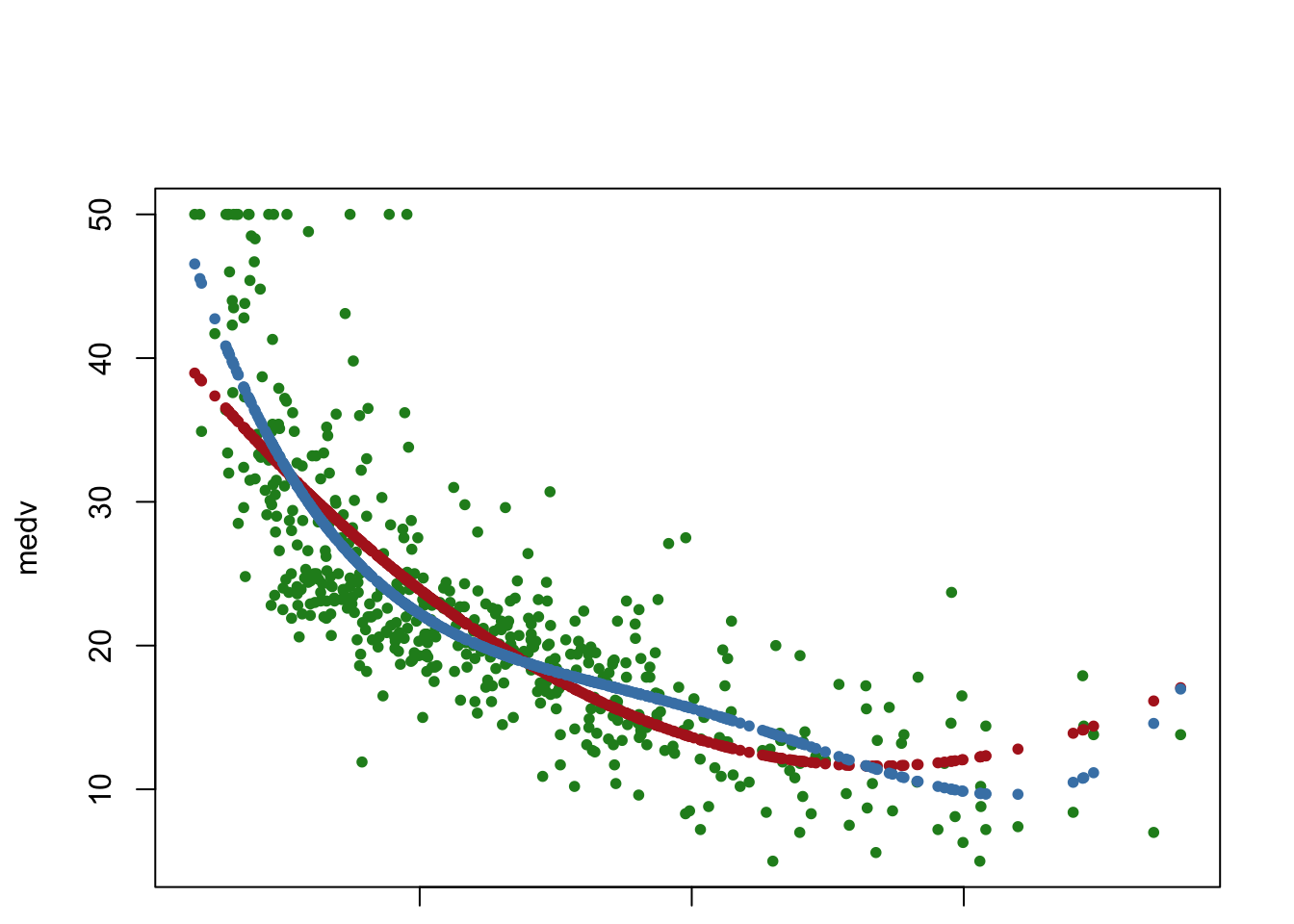
## I() identity function for squared term to interpret as-is## Combine two command lines with semicolonfit6=lm(medv~lstat +I(lstat^2),Boston); summary(fit6)
Call:
lm(formula = medv ~ lstat + I(lstat^2), data = Boston)

Residuals:
     Min       1Q   Median       3Q      Max
-15.2834  -3.8313  -0.5295   2.3095  25.4148

Coefficients:
             Estimate Std. Error t value Pr(>|t|)
(Intercept) 42.862007   0.872084   49.15   <2e-16 ***
lstat       -2.332821   0.123803  -18.84   <2e-16 ***
I(lstat^2)   0.043547   0.003745   11.63   <2e-16 ***
---
Signif. codes:  0 '***' 0.001 '**' 0.01 '*' 0.05 '.' 0.1 ' ' 1

Residual standard error: 5.524 on 503 degrees of freedom
Multiple R-squared:  0.6407,    Adjusted R-squared:  0.6393
F-statistic: 448.5 on 2 and 503 DF,  p-value: < 2.2e-16
     Sales          CompPrice       Income        Advertising
 Min.   : 0.000   Min.   : 77   Min.   : 21.00   Min.   : 0.000
 1st Qu.: 5.390   1st Qu.:115   1st Qu.: 42.75   1st Qu.: 0.000
 Median : 7.490   Median :125   Median : 69.00   Median : 5.000
 Mean   : 7.496   Mean   :125   Mean   : 68.66   Mean   : 6.635
 3rd Qu.: 9.320   3rd Qu.:135   3rd Qu.: 91.00   3rd Qu.:12.000
 Max.   :16.270   Max.   :175   Max.   :120.00   Max.   :29.000
   Population        Price        ShelveLoc        Age          Education
 Min.   : 10.0   Min.   : 24.0   Bad   : 96   Min.   :25.00   Min.   :10.0
 1st Qu.:139.0   1st Qu.:100.0   Good  : 85   1st Qu.:39.75   1st Qu.:12.0
 Median :272.0   Median :117.0   Medium:219   Median :54.50   Median :14.0
 Mean   :264.8   Mean   :115.8                Mean   :53.32   Mean   :13.9
 3rd Qu.:398.5   3rd Qu.:131.0                3rd Qu.:66.00   3rd Qu.:16.0
 Max.   :509.0   Max.   :191.0                Max.   :80.00   Max.   :18.0
 Urban       US
 No :118   No :142
 Yes:282   Yes:258
fit1=lm(Sales~.+Income:Advertising+Age:Price,Carseats) # add two interaction termssummary(fit1)
attach(Carseats)contrasts(Carseats$ShelveLoc) # what is contrasts function?
       Good Medium
Bad       0      0
Good      1      0
Medium    0      1
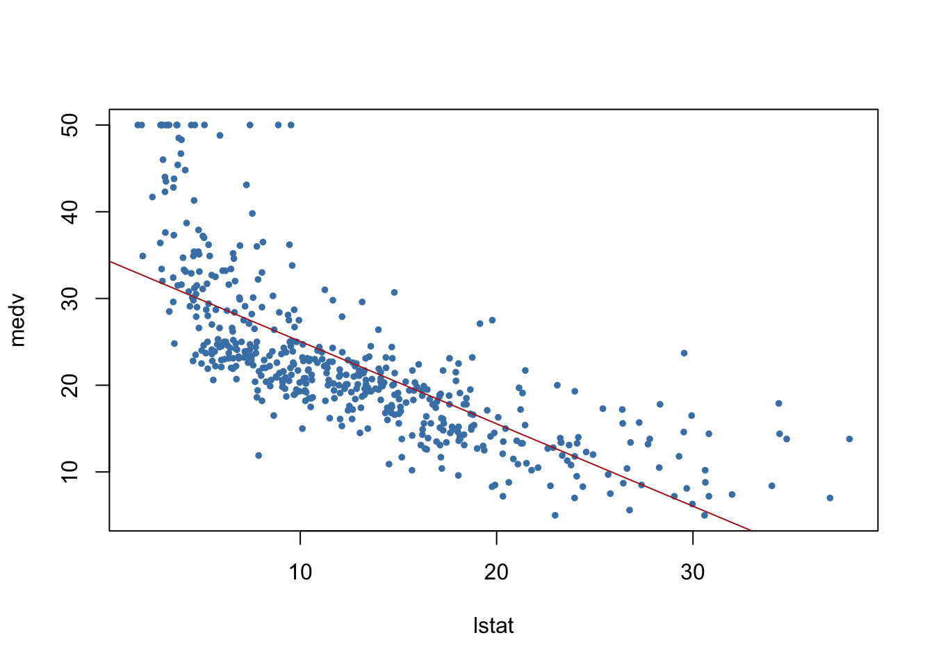
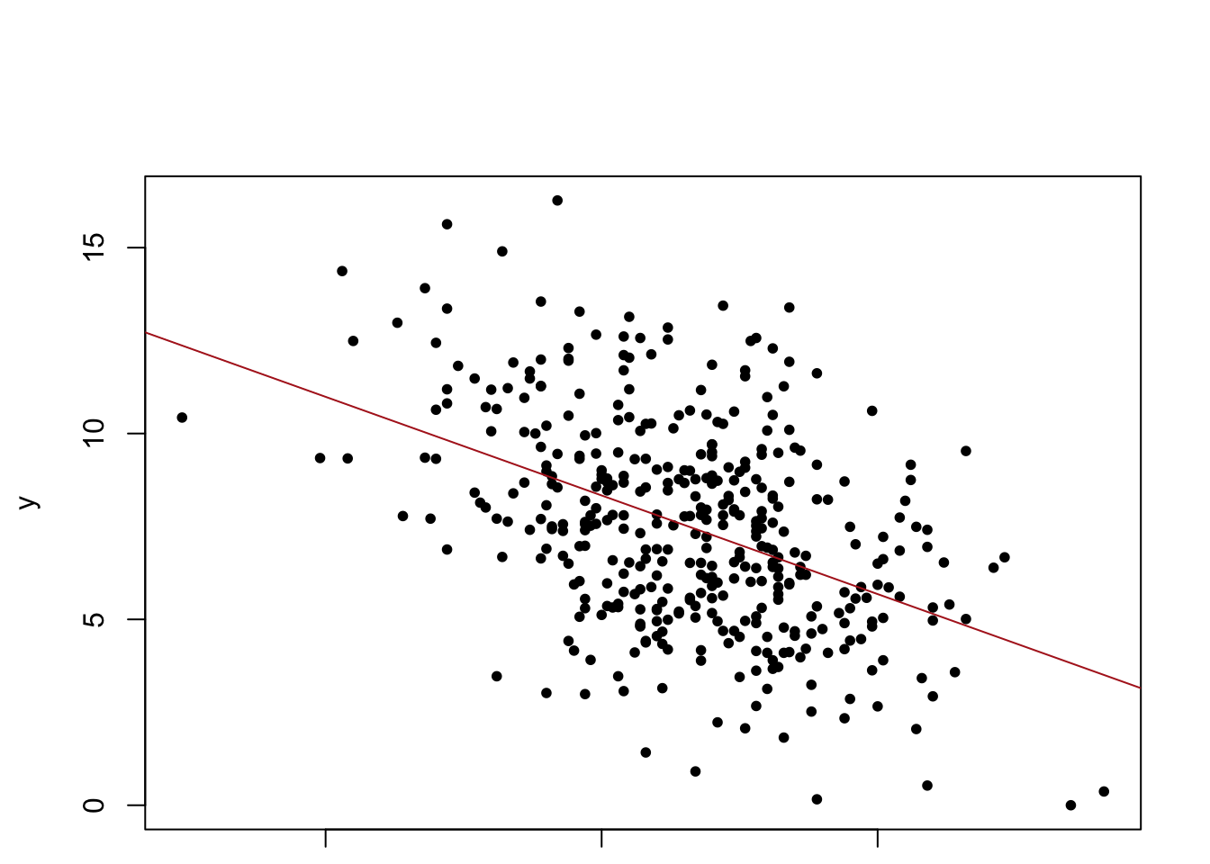
?contrasts### Writing an R function to combine the lm, plot and abline functions to ### create a one step regression fit plot functionregplot=function(x,y){ fit=lm(y~x)plot(x,y, pch=20)abline(fit,col="firebrick")}attach(Carseats)
The following objects are masked from Carseats (pos = 3):

    Advertising, Age, CompPrice, Education, Income, Population, Price,
    Sales, ShelveLoc, Urban, US
regplot(Price,Sales)
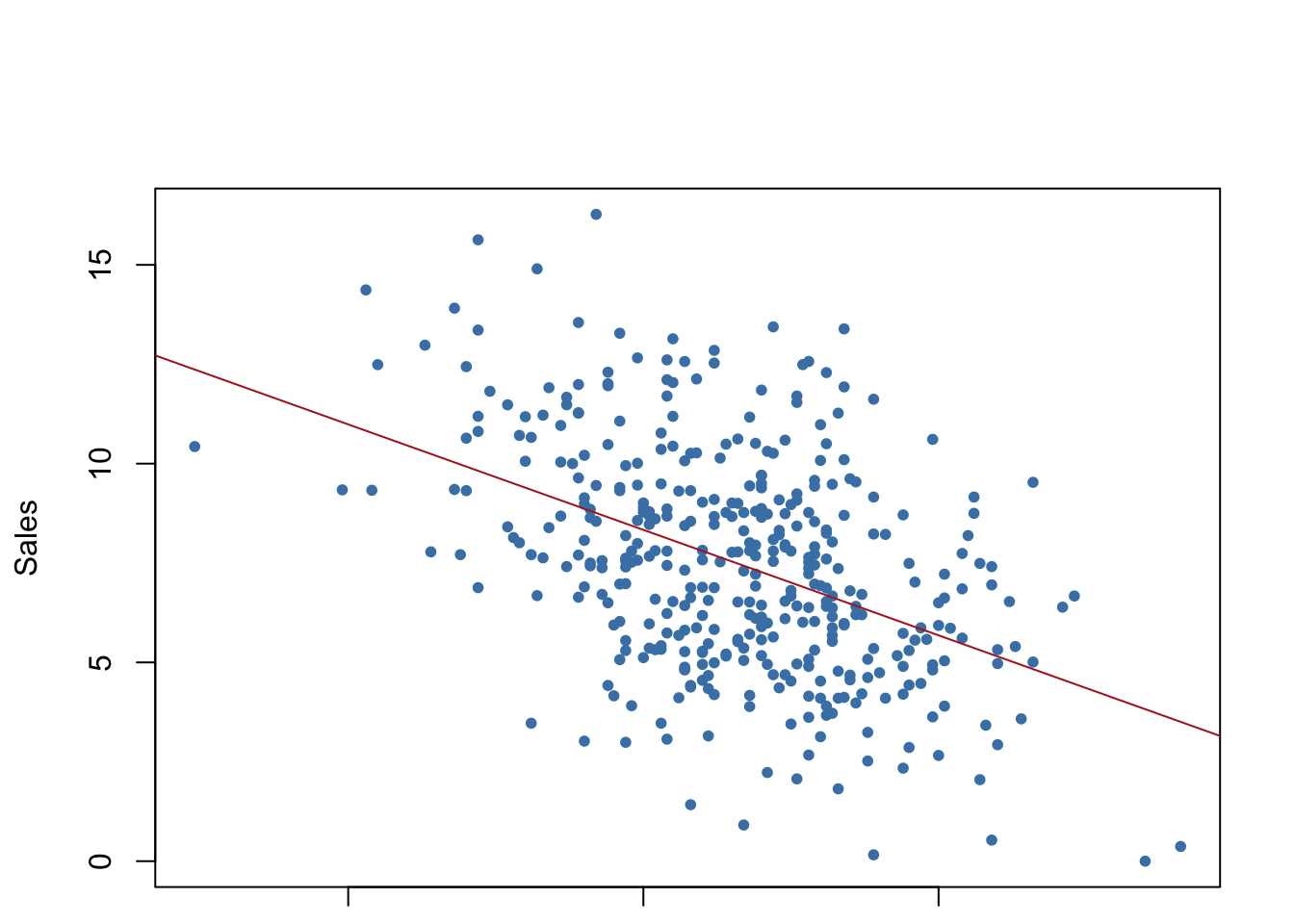
## Allow extra room for additional arguments/specificationsregplot=function(x,y,...){ fit=lm(y~x)plot(x,y,...)abline(fit,col="firebrick")}regplot(Price,Sales,xlab="Price",ylab="Sales",col="steelblue",pch=20)
## Additional note: try out the coefplot2 package to finetune the coefplotsinstall.packages("coefplot2", repos="http://www.math.mcmaster.ca/bolker/R", type="source")remotes::install_github("palday/coefplot2", subdir ="pkg")
Downloading GitHub repo palday/coefplot2@HEAD
rlang (1.1.0 -> 1.1.1) [CRAN]
Installing 1 packages: rlang
  There is a binary version available but the source version is later:
      binary source needs_compilation
rlang  1.1.0  1.1.1              TRUE
installing the source package 'rlang'
── R CMD build ─────────────────────────────────────────────────────────────────
* checking for file ‘/private/var/folders/fg/l9nwkw5954b_7xv794xmt5_40000gn/T/Rtmps29Aev/remotesd732e16f41c/palday-coefplot2-23b7dcb/pkg/DESCRIPTION’ ... OK
* preparing ‘coefplot2’:
* checking DESCRIPTION meta-information ... OK
* checking for LF line-endings in source and make files and shell scripts
* checking for empty or unneeded directories
* building ‘coefplot2_0.1.3.3.tar.gz’
library(coefplot2)
Loading required package: coda
Attaching package: 'coda'
The following object is masked from 'package:arm':

    traceplot
coefplot2(fit3)
Part 2
Use the TEDS2016 dataset to run a logit (logistic regression) model using female as sole predictor. The dependent variable is the vote (1-0) for Tsai Ing-wen, the female candidate for the then opposition party Democratic Progressive Party (DPP).
Call:
glm(formula = votetsai ~ female, family = binomial, data = TEDS_2016)

Deviance Residuals:
    Min       1Q   Median       3Q      Max
-1.4180  -1.3889   0.9546   0.9797   0.9797

Coefficients:
            Estimate Std. Error z value Pr(>|z|)
(Intercept)  0.54971    0.08245   6.667 2.61e-11 ***
female      -0.06517    0.11644  -0.560    0.576
---
Signif. codes:  0 '***' 0.001 '**' 0.01 '*' 0.05 '.' 0.1 ' ' 1

(Dispersion parameter for binomial family taken to be 1)

    Null deviance: 1666.5  on 1260  degrees of freedom
Residual deviance: 1666.2  on 1259  degrees of freedom
  (429 observations deleted due to missingness)
AIC: 1670.2

Number of Fisher Scoring iterations: 4
Are female voters more likely to vote for President Tsai? Why or why not? No because the value for the coefficient for the female variable is -0.06517 which is not significant. Suggesting there are no differences between male and female voters.
Add party ID variables (KMT, DPP) and other demographic variables (age, edu, income) to improve the model. What do you find? Which group of variables work better in explaining/predicting votetsai?
glm.vt2 <-glm(votetsai~female + KMT + DPP + age + edu + income, data=TEDS_2016,family=binomial)summary(glm.vt2)
Call:
glm(formula = votetsai ~ female + KMT + DPP + age + edu + income,
    family = binomial, data = TEDS_2016)

Deviance Residuals:
    Min       1Q   Median       3Q      Max
-2.7360  -0.3673   0.2408   0.2946   2.5408

Coefficients:
             Estimate Std. Error z value Pr(>|z|)
(Intercept)  1.618640   0.592084   2.734  0.00626 **
female       0.047406   0.177403   0.267  0.78930
KMT         -3.156273   0.250360 -12.607  < 2e-16 ***
DPP          2.888943   0.267968  10.781  < 2e-16 ***
age         -0.011808   0.007164  -1.648  0.09931 .
edu         -0.184604   0.083102  -2.221  0.02632 *
income       0.013727   0.034382   0.399  0.68971
---
Signif. codes:  0 '***' 0.001 '**' 0.01 '*' 0.05 '.' 0.1 ' ' 1

(Dispersion parameter for binomial family taken to be 1)

    Null deviance: 1661.76  on 1256  degrees of freedom
Residual deviance:  836.15  on 1250  degrees of freedom
  (433 observations deleted due to missingness)
AIC: 850.15

Number of Fisher Scoring iterations: 6
In this, it seems that KMT and DPP predict votesai better (AIC = 850). When using female as the predictor the AIC was 1670. A lower AIC value shows the better fit. (AIC = Akaike Information Criterion).
Try adding the following variables: Independence – Supporting Taiwan’s Independence (vs. Unification with China), Econ_worse – Evaluations of economy (Negative), Govt_dont_care – Political Efficacy (Government does not care about people), Minnan_father – Descendent of local Taiwanese, Mainland_father – Descendent of mainland China (migrated from mainland circa or after 1949), Taiwanese – Self-identified Taiwanese
glm.vt3 <-glm(votetsai~female + KMT + DPP + age + edu + income + Independence + Econ_worse + Govt_dont_care + Minnan_father + Mainland_father + Taiwanese, data=TEDS_2016,family=binomial)summary(glm.vt3)
Call:
glm(formula = votetsai ~ female + KMT + DPP + age + edu + income +
    Independence + Econ_worse + Govt_dont_care + Minnan_father +
    Mainland_father + Taiwanese, family = binomial, data = TEDS_2016)

Deviance Residuals:
    Min       1Q   Median       3Q      Max
-3.1060  -0.3143   0.1744   0.3975   2.7917

Coefficients:
                 Estimate Std. Error z value Pr(>|z|)
(Intercept)     -0.015976   0.679780  -0.024  0.98125
female          -0.097996   0.189840  -0.516  0.60571
KMT             -2.922246   0.259333 -11.268  < 2e-16 ***
DPP              2.468855   0.275350   8.966  < 2e-16 ***
age              0.003287   0.007884   0.417  0.67672
edu             -0.092110   0.090119  -1.022  0.30674
income           0.021771   0.036406   0.598  0.54984
Independence     1.020953   0.251776   4.055 5.01e-05 ***
Econ_worse       0.310462   0.189100   1.642  0.10063
Govt_dont_care  -0.014295   0.188765  -0.076  0.93964
Minnan_father   -0.247650   0.253921  -0.975  0.32941
Mainland_father -1.089332   0.396822  -2.745  0.00605 **
Taiwanese        0.909019   0.198930   4.570 4.89e-06 ***
---
Signif. codes:  0 '***' 0.001 '**' 0.01 '*' 0.05 '.' 0.1 ' ' 1

(Dispersion parameter for binomial family taken to be 1)

    Null deviance: 1661.76  on 1256  degrees of freedom
Residual deviance:  767.13  on 1244  degrees of freedom
  (433 observations deleted due to missingness)
AIC: 793.13

Number of Fisher Scoring iterations: 6
Here the AIC for the model is 793.13, suggesting that the model with these variables added is the best for predicting votesai