assignment04

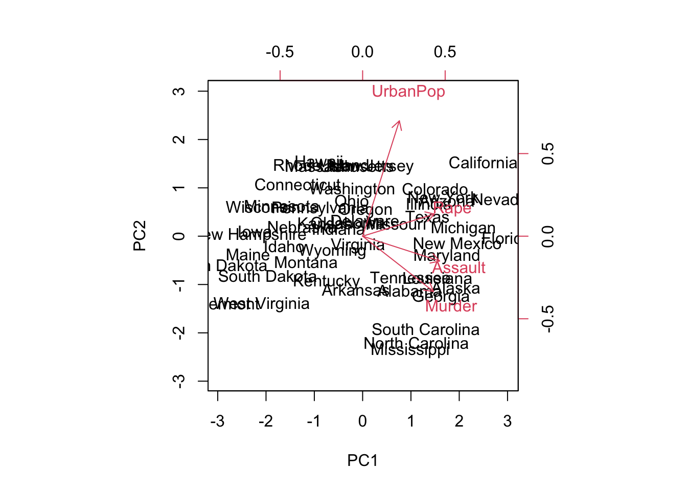
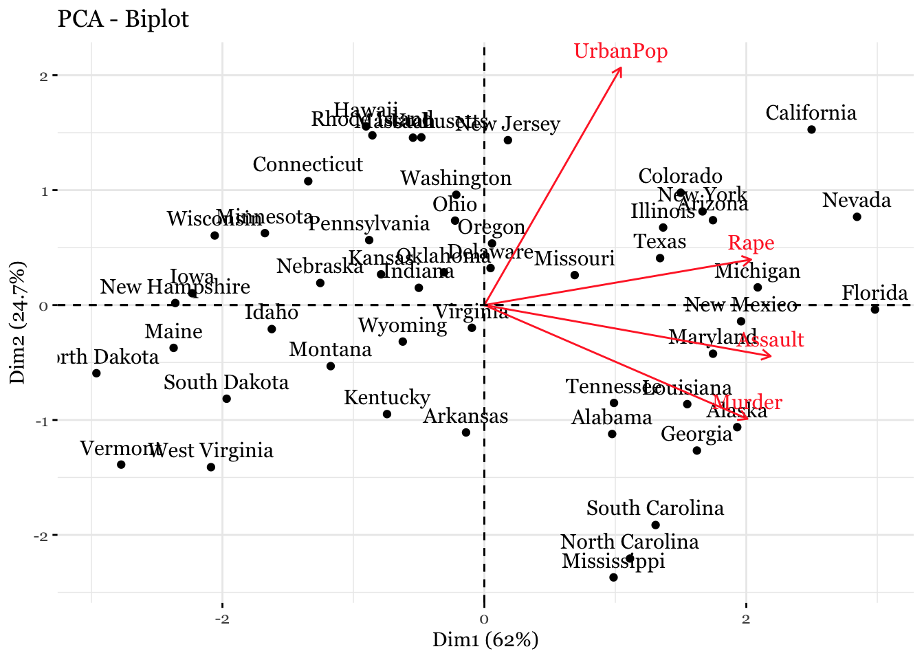
## Gentle Machine Learning
## Principal Component Analysis


# Dataset: USArrests is the sample dataset used in 
# McNeil, D. R. (1977) Interactive Data Analysis. New York: Wiley.
# Murder    numeric Murder arrests (per 100,000)
# Assault   numeric Assault arrests (per 100,000)
# UrbanPop  numeric Percent urban population
# Rape  numeric Rape arrests (per 100,000)
# For each of the fifty states in the United States, the dataset contains the number 
# of arrests per 100,000 residents for each of three crimes: Assault, Murder, and Rape. 
# UrbanPop is the percent of the population in each state living in urban areas.
library(datasets)
library(ISLR)
arrest = USArrests
states=row.names(USArrests)
names(USArrests)

[1] "Murder"   "Assault"  "UrbanPop" "Rape"    

# Get means and variances of variables
apply(USArrests, 2, mean)

  Murder  Assault UrbanPop     Rape 
   7.788  170.760   65.540   21.232 

apply(USArrests, 2, var)

    Murder    Assault   UrbanPop       Rape 
  18.97047 6945.16571  209.51878   87.72916 

# PCA with scaling
pr.out=prcomp(USArrests, scale=TRUE)
names(pr.out) # Five

[1] "sdev"     "rotation" "center"   "scale"    "x"       

pr.out$center # the centering and scaling used (means)

  Murder  Assault UrbanPop     Rape 
   7.788  170.760   65.540   21.232 

pr.out$scale # the matrix of variable loadings (eigenvectors)

   Murder   Assault  UrbanPop      Rape 
 4.355510 83.337661 14.474763  9.366385 

pr.out$rotation

                PC1        PC2        PC3         PC4
Murder   -0.5358995  0.4181809 -0.3412327  0.64922780
Assault  -0.5831836  0.1879856 -0.2681484 -0.74340748
UrbanPop -0.2781909 -0.8728062 -0.3780158  0.13387773
Rape     -0.5434321 -0.1673186  0.8177779  0.08902432

dim(pr.out$x)

[1] 50  4

pr.out$rotation=-pr.out$rotation
pr.out$x=-pr.out$x
biplot(pr.out, scale=0)

pr.out$sdev

[1] 1.5748783 0.9948694 0.5971291 0.4164494

pr.var=pr.out$sdev^2
pr.var

[1] 2.4802416 0.9897652 0.3565632 0.1734301

pve=pr.var/sum(pr.var)
pve

[1] 0.62006039 0.24744129 0.08914080 0.04335752

plot(pve, xlab="Principal Component", ylab="Proportion of Variance Explained", ylim=c(0,1),type='b')

plot(cumsum(pve), xlab="Principal Component", ylab="Cumulative Proportion of Variance Explained", ylim=c(0,1),type='b')

## Use factoextra package
library(factoextra)

Loading required package: ggplot2

Welcome! Want to learn more? See two factoextra-related books at https://goo.gl/ve3WBa

fviz(pr.out, "ind", geom = "auto", mean.point = TRUE, font.family = "Georgia")

fviz_pca_biplot(pr.out, font.family = "Georgia", col.var="firebrick1")

## Computer purchase example: Animated illustration 
## Adapted from Guru99 tutorial (https://www.guru99.com/r-k-means-clustering.html)
## Dataset: characteristics of computers purchased.
## Variables used: RAM size, Harddrive size

library(dplyr)

Attaching package: 'dplyr'

The following objects are masked from 'package:stats':

    filter, lag

The following objects are masked from 'package:base':

    intersect, setdiff, setequal, union

library(ggplot2)
library(RColorBrewer)

computers = read.csv("https://raw.githubusercontent.com/guru99-edu/R-Programming/master/computers.csv") 

# Only retain two variables for illustration
rescaled_comp <- computers[4:5] %>%
  mutate(hd_scal = scale(hd),
         ram_scal = scale(ram)) %>%
  select(c(hd_scal, ram_scal))
        
ggplot(data = rescaled_comp, aes(x = hd_scal, y = ram_scal)) +
  geom_point(pch=20, col = "blue") + theme_bw() +
  labs(x = "Hard drive size (Scaled)", y ="RAM size (Scaled)" ) +
  theme(text = element_text(family="Georgia")) 

install.packages('animation', repos = 'http://rforge.net', type = 'source')

# install.packages("animation")
library(animation)
set.seed(2345)
library(animation)

# Animate the K-mean clustering process, cluster no. = 4
kmeans.ani(rescaled_comp[1:2], centers = 4, pch = 15:18, col = 1:4) 

saveGIF(
  kmeans.ani(rescaled_comp[1:2], centers = 4, pch = 15:18, col = 1:4) ,
  movie.name = "kmeans_animated.gif",
  img.name = "kmeans",
  convert = "magick",
  cmd.fun,
  clean = TRUE,
  extra.opts = ""
)

Output at: kmeans_animated.gif

[1] TRUE

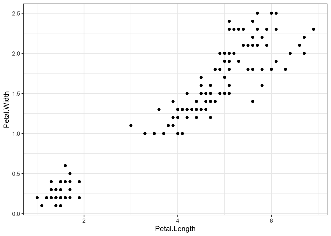
## Iris example

# Without grouping by species
ggplot(iris, aes(Petal.Length, Petal.Width)) + geom_point() + 
  theme_bw() +
  scale_color_manual(values=c("firebrick1","forestgreen","darkblue"))

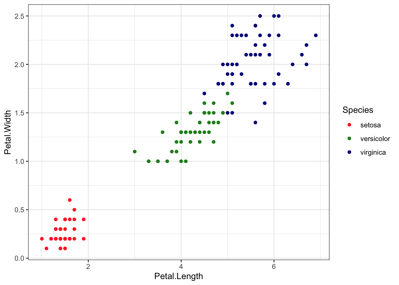
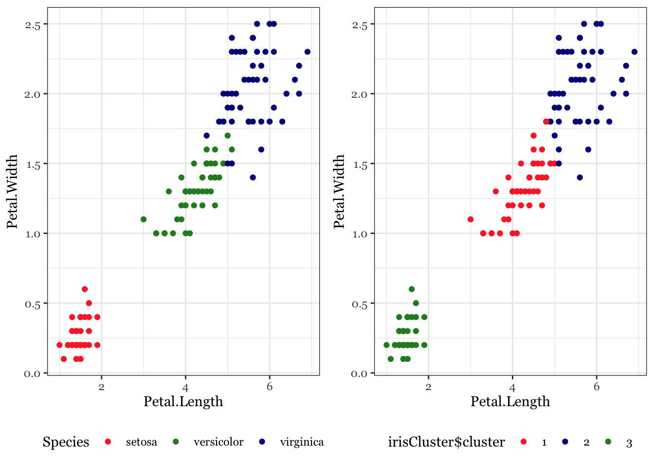
# With grouping by species
ggplot(iris, aes(Petal.Length, Petal.Width, color = Species)) + geom_point() + 
  theme_bw() +
  scale_color_manual(values=c("firebrick1","forestgreen","darkblue"))

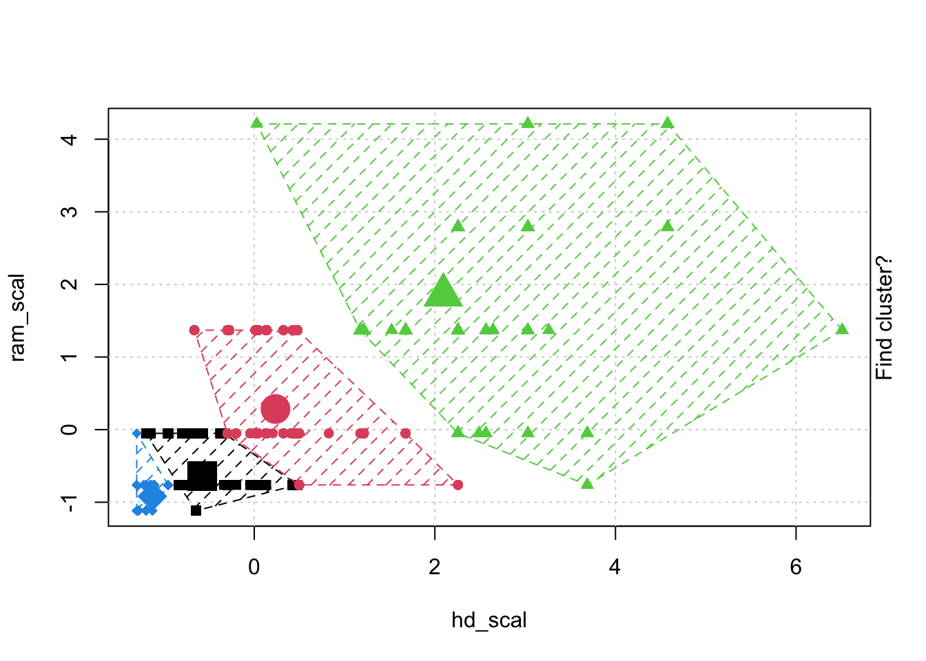
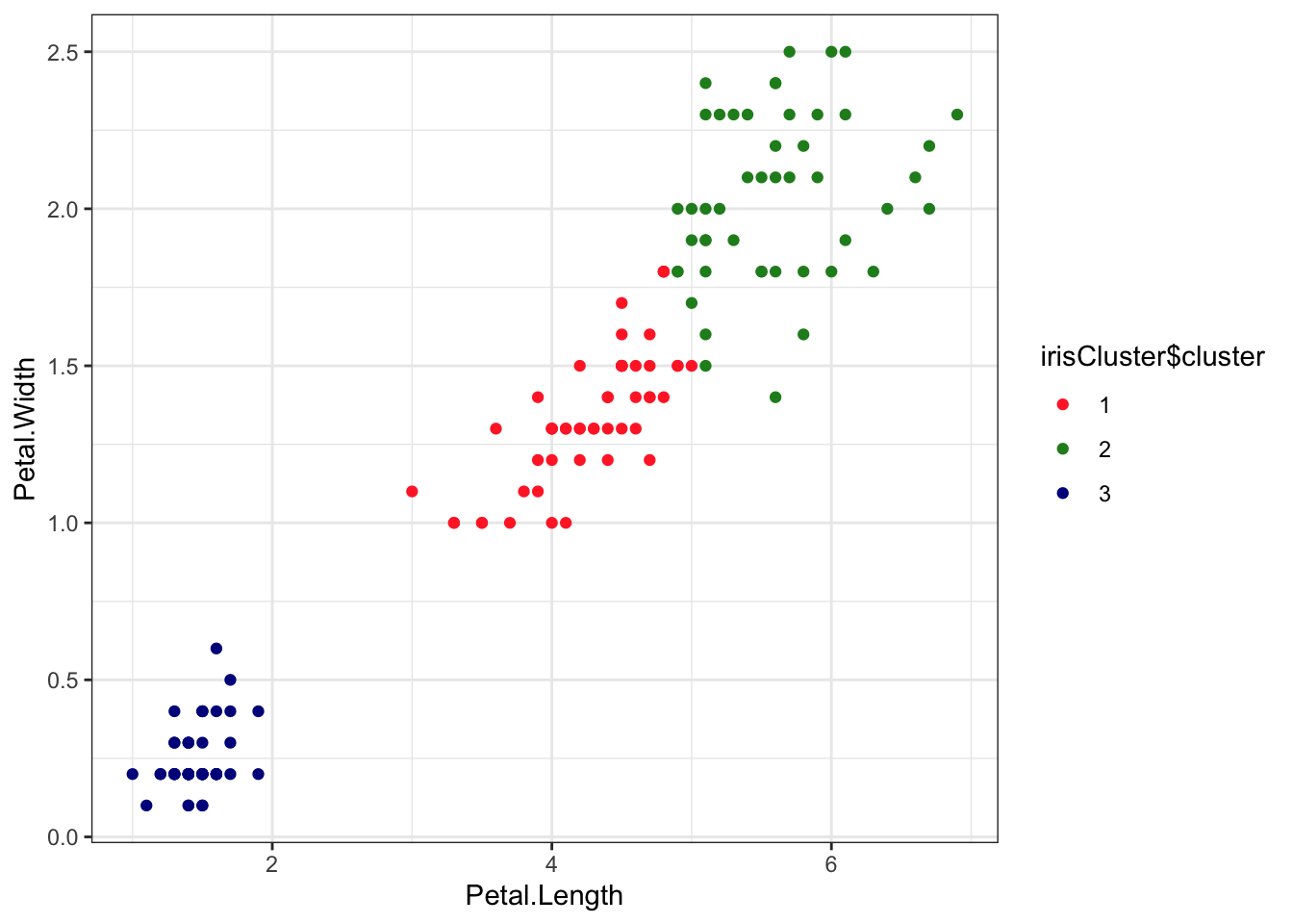
# Check k-means clusters
## Starting with three clusters and 20 initial configurations
set.seed(20)
irisCluster <- kmeans(iris[, 3:4], 3, nstart = 20)
irisCluster

K-means clustering with 3 clusters of sizes 52, 48, 50

Cluster means:
  Petal.Length Petal.Width
1     4.269231    1.342308
2     5.595833    2.037500
3     1.462000    0.246000

Clustering vector:
  [1] 3 3 3 3 3 3 3 3 3 3 3 3 3 3 3 3 3 3 3 3 3 3 3 3 3 3 3 3 3 3 3 3 3 3 3 3 3
 [38] 3 3 3 3 3 3 3 3 3 3 3 3 3 1 1 1 1 1 1 1 1 1 1 1 1 1 1 1 1 1 1 1 1 1 1 1 1
 [75] 1 1 1 2 1 1 1 1 1 2 1 1 1 1 1 1 1 1 1 1 1 1 1 1 1 1 2 2 2 2 2 2 1 2 2 2 2
[112] 2 2 2 2 2 2 2 2 1 2 2 2 2 2 2 1 2 2 2 2 2 2 2 2 2 2 2 1 2 2 2 2 2 2 2 2 2
[149] 2 2

Within cluster sum of squares by cluster:
[1] 13.05769 16.29167  2.02200
 (between_SS / total_SS =  94.3 %)

Available components:

[1] "cluster"      "centers"      "totss"        "withinss"     "tot.withinss"
[6] "betweenss"    "size"         "iter"         "ifault"      

class(irisCluster$cluster)

[1] "integer"

# Confusion matrix
table(irisCluster$cluster, iris$Species)

   
    setosa versicolor virginica
  1      0         48         4
  2      0          2        46
  3     50          0         0

irisCluster$cluster <- as.factor(irisCluster$cluster)
ggplot(iris, aes(Petal.Length, Petal.Width, color = irisCluster$cluster)) + geom_point() +
  scale_color_manual(values=c("firebrick1","forestgreen","darkblue")) +
  theme_bw()

actual = ggplot(iris, aes(Petal.Length, Petal.Width, color = Species)) + geom_point() + 
  theme_bw() +
  scale_color_manual(values=c("firebrick1","forestgreen","darkblue")) +
  theme(legend.position="bottom") +
  theme(text = element_text(family="Georgia")) 
kmc = ggplot(iris, aes(Petal.Length, Petal.Width, color = irisCluster$cluster)) + geom_point() +
  theme_bw() +
  scale_color_manual(values=c("firebrick1", "darkblue", "forestgreen")) +
  theme(legend.position="bottom") +
  theme(text = element_text(family="Georgia")) 
library(grid)
library(gridExtra)

Attaching package: 'gridExtra'

The following object is masked from 'package:dplyr':

    combine

grid.arrange(arrangeGrob(actual, kmc, ncol=2, widths=c(1,1)), nrow=1)

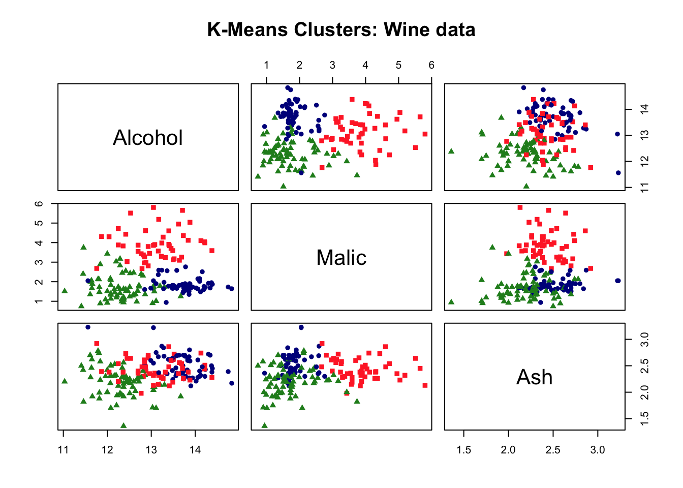
## Wine example

# The wine dataset contains the results of a chemical analysis of wines 
# grown in a specific area of Italy. Three types of wine are represented in the 
# 178 samples, with the results of 13 chemical analyses recorded for each sample. 
# Variables used in this example:
# Alcohol
# Malic: Malic acid
# Ash
# Source: http://archive.ics.uci.edu/ml/datasets/Wine

# Import wine dataset
library(readr)
wine <- read_csv("https://raw.githubusercontent.com/datageneration/gentlemachinelearning/master/data/wine.csv")

Rows: 178 Columns: 14
── Column specification ────────────────────────────────────────────────────────
Delimiter: ","
dbl (14): class, Alcohol, Malic, Ash, Ash_alcalinity, Magnesium, Total_pheno...

ℹ Use `spec()` to retrieve the full column specification for this data.
ℹ Specify the column types or set `show_col_types = FALSE` to quiet this message.

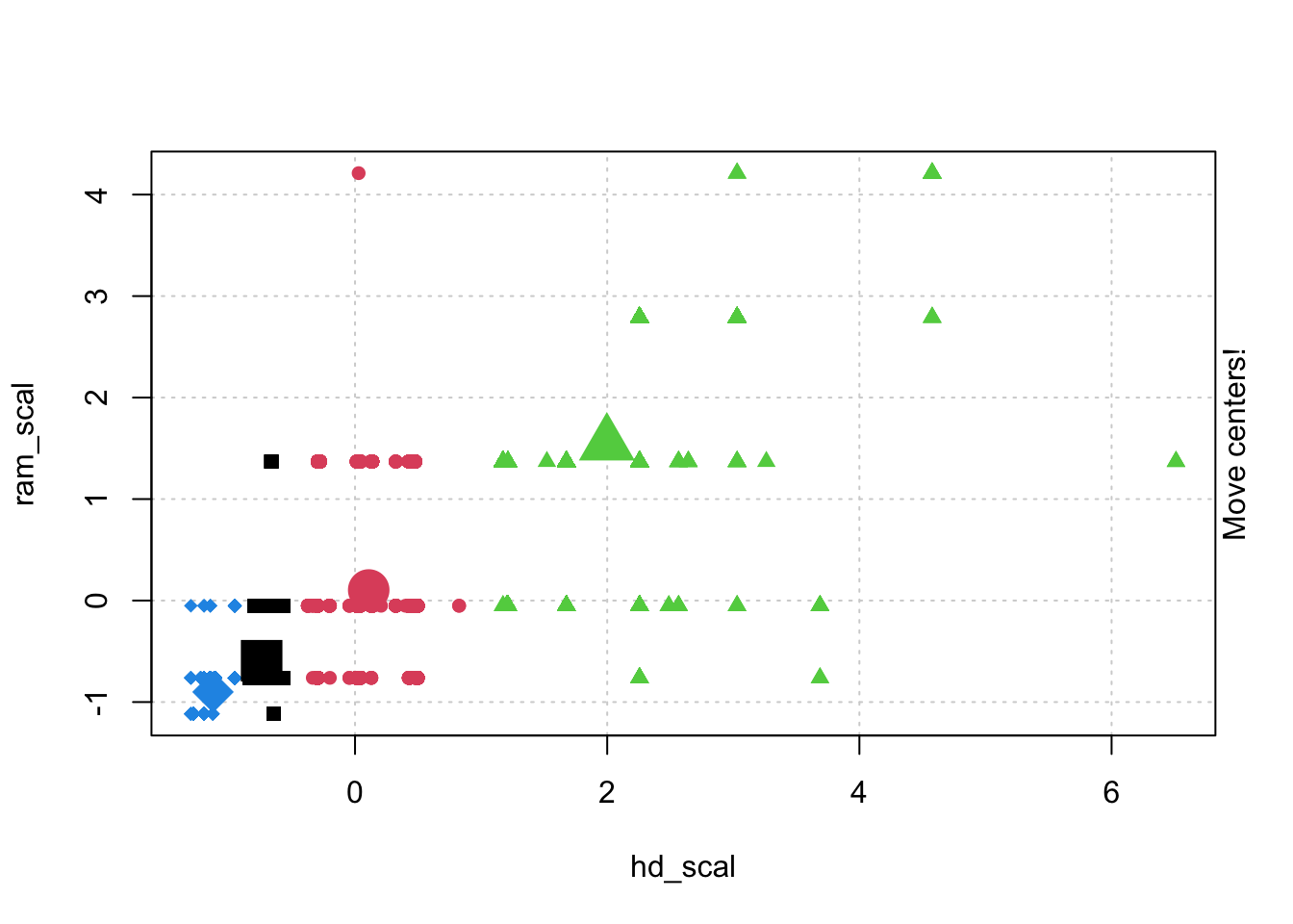
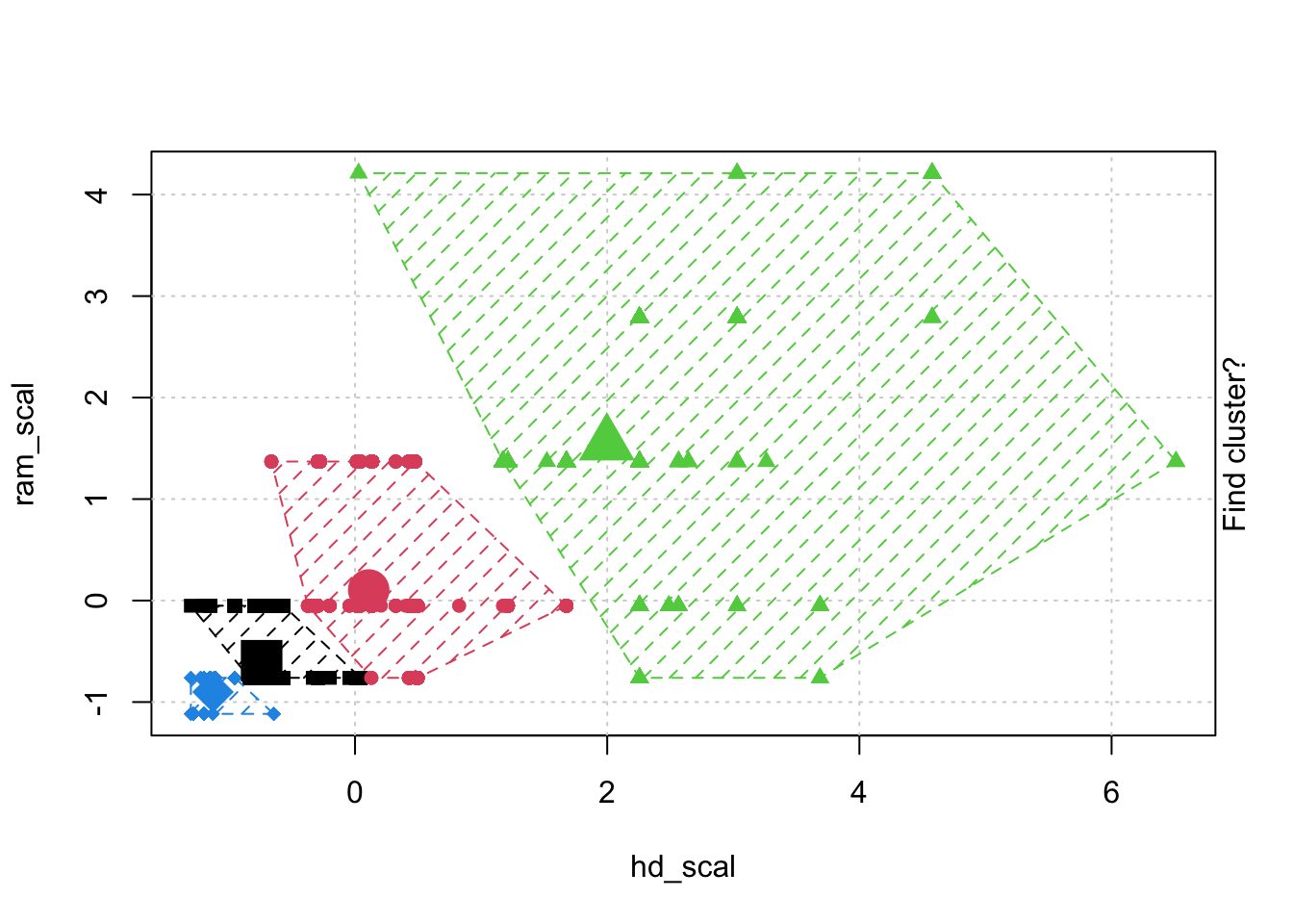
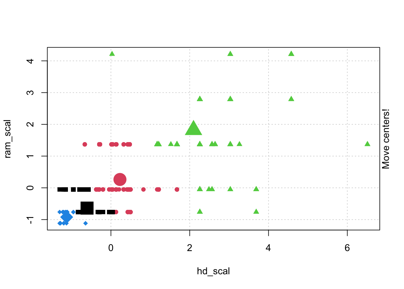
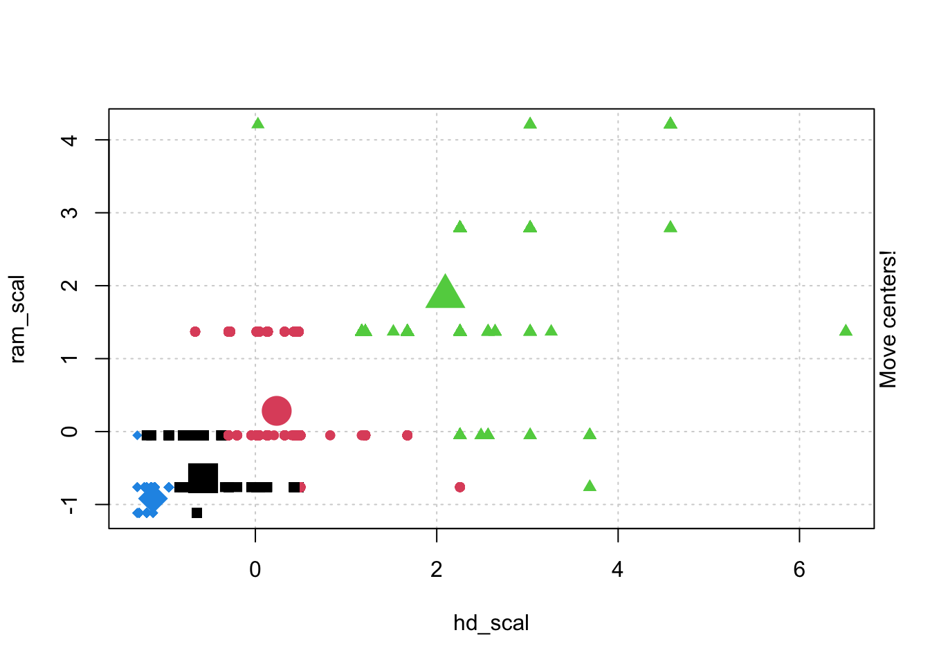
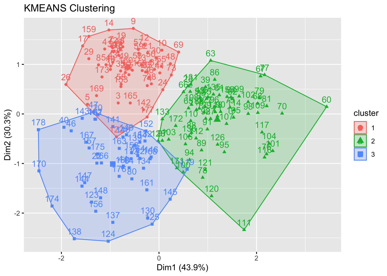
## Choose and scale variables
wine_subset <- scale(wine[ , c(2:4)])

## Create cluster using k-means, k = 3, with 25 initial configurations
wine_cluster <- kmeans(wine_subset, centers = 3,
                       iter.max = 10,
                       nstart = 25)
wine_cluster

K-means clustering with 3 clusters of sizes 48, 60, 70

Cluster means:
     Alcohol      Malic        Ash
1  0.1470536  1.3907328  0.2534220
2  0.8914655 -0.4522073  0.5406223
3 -0.8649501 -0.5660390 -0.6371656

Clustering vector:
  [1] 2 3 2 2 2 2 2 2 2 2 2 2 2 2 2 2 2 2 2 1 2 1 2 2 2 2 2 3 2 2 2 2 2 2 2 2 2
 [38] 2 3 1 2 1 2 1 3 1 1 2 2 2 3 2 2 2 2 2 2 2 2 3 3 3 3 3 3 3 3 3 2 3 3 2 2 2
 [75] 3 3 3 3 3 1 3 3 3 1 3 3 3 3 3 3 3 3 3 3 3 3 3 3 3 3 3 3 3 3 3 3 3 3 3 3 3
[112] 3 1 3 3 3 3 3 1 3 3 2 1 1 1 3 3 3 3 1 3 1 3 1 3 3 1 1 1 1 1 2 1 1 1 1 1 1
[149] 1 1 1 1 2 1 3 1 1 1 2 2 1 1 1 1 2 1 1 1 2 1 3 3 2 1 1 1 2 1

Within cluster sum of squares by cluster:
[1]  73.71460  67.98619 111.63512
 (between_SS / total_SS =  52.3 %)

Available components:

[1] "cluster"      "centers"      "totss"        "withinss"     "tot.withinss"
[6] "betweenss"    "size"         "iter"         "ifault"      

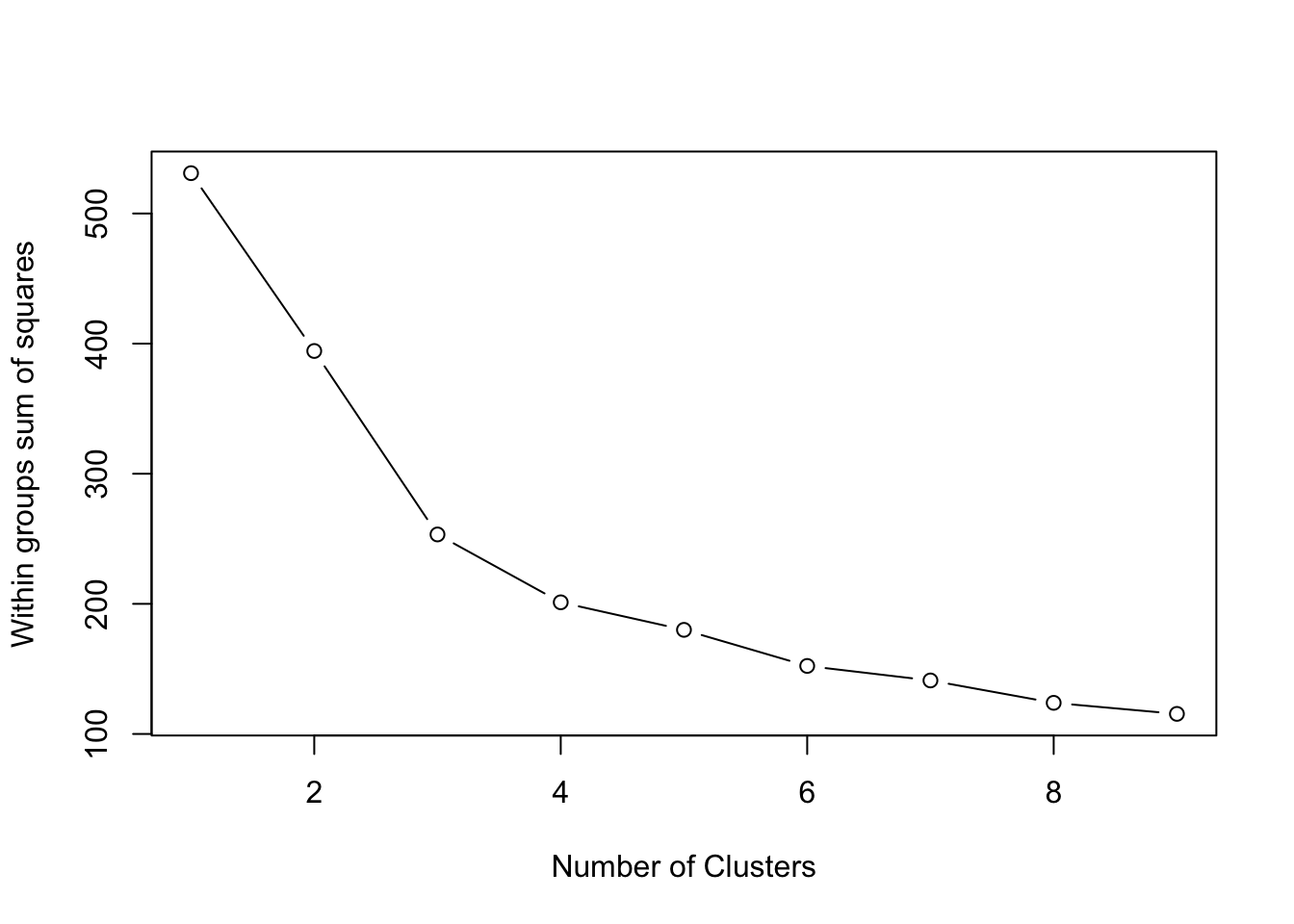
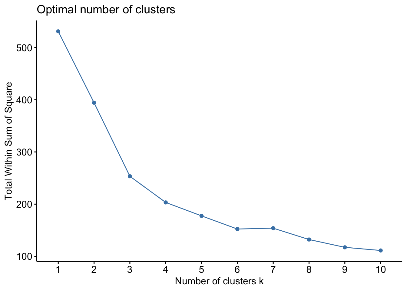
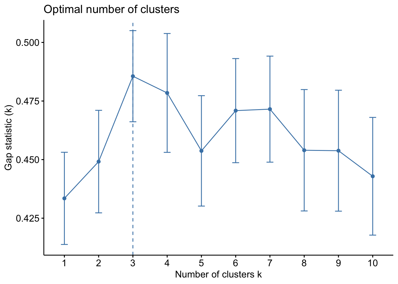
# Create a function to compute and plot total within-cluster sum of square (within-ness)
wssplot <- function(data, nc=15, seed=1234){
  wss <- (nrow(data)-1)*sum(apply(data,2,var))
  for (i in 2:nc){
    set.seed(seed)
    wss[i] <- sum(kmeans(data, centers=i)$withinss)}
  plot(1:nc, wss, type="b", xlab="Number of Clusters",
       ylab="Within groups sum of squares")
}

# plotting values for each cluster starting from 1 to 9
wssplot(wine_subset, nc = 9)

# Plot results by dimensions
wine_cluster$cluster = as.factor(wine_cluster$cluster)
pairs(wine[2:4],
      col = c("firebrick1", "darkblue", "forestgreen")[wine_cluster$cluster],
      pch = c(15:17)[wine_cluster$cluster],
      main = "K-Means Clusters: Wine data")

table(wine_cluster$cluster)

 1  2  3 
48 60 70 

## Use the factoextra package to do more

library(factoextra)
fviz_nbclust(wine_subset, kmeans, method = "wss")

# Use eclust() procedure to do K-Means
wine.km <- eclust(wine_subset, "kmeans", nboot = 2)

# Print result
wine.km

K-means clustering with 3 clusters of sizes 60, 70, 48

Cluster means:
     Alcohol      Malic        Ash
1  0.8914655 -0.4522073  0.5406223
2 -0.8649501 -0.5660390 -0.6371656
3  0.1470536  1.3907328  0.2534220

Clustering vector:
  [1] 1 2 1 1 1 1 1 1 1 1 1 1 1 1 1 1 1 1 1 3 1 3 1 1 1 1 1 2 1 1 1 1 1 1 1 1 1
 [38] 1 2 3 1 3 1 3 2 3 3 1 1 1 2 1 1 1 1 1 1 1 1 2 2 2 2 2 2 2 2 2 1 2 2 1 1 1
 [75] 2 2 2 2 2 3 2 2 2 3 2 2 2 2 2 2 2 2 2 2 2 2 2 2 2 2 2 2 2 2 2 2 2 2 2 2 2
[112] 2 3 2 2 2 2 2 3 2 2 1 3 3 3 2 2 2 2 3 2 3 2 3 2 2 3 3 3 3 3 1 3 3 3 3 3 3
[149] 3 3 3 3 1 3 2 3 3 3 1 1 3 3 3 3 1 3 3 3 1 3 2 2 1 3 3 3 1 3

Within cluster sum of squares by cluster:
[1]  67.98619 111.63512  73.71460
 (between_SS / total_SS =  52.3 %)

Available components:

 [1] "cluster"      "centers"      "totss"        "withinss"     "tot.withinss"
 [6] "betweenss"    "size"         "iter"         "ifault"       "clust_plot"  
[11] "silinfo"      "nbclust"      "data"         "gap_stat"    

# Optimal number of clusters using gap statistics
wine.km$nbclust

[1] 3

fviz_nbclust(wine_subset, kmeans, method = "gap_stat")

# Silhouette plot
fviz_silhouette(wine.km)

  cluster size ave.sil.width
1       1   60          0.44
2       2   70          0.33
3       3   48          0.30

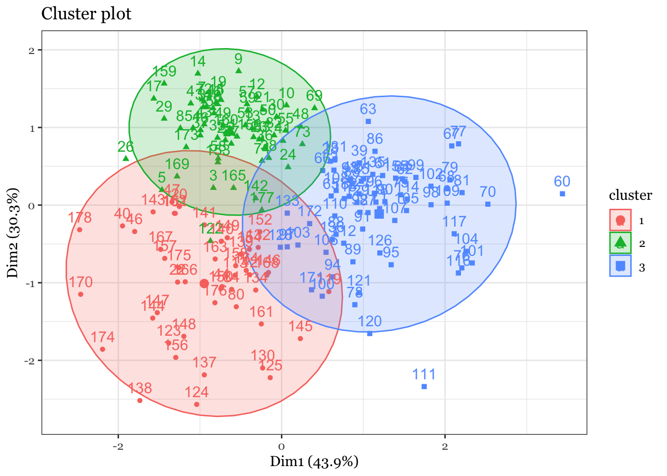
fviz_cluster(wine_cluster, data = wine_subset) + 
  theme_bw() +
  theme(text = element_text(family="Georgia")) 

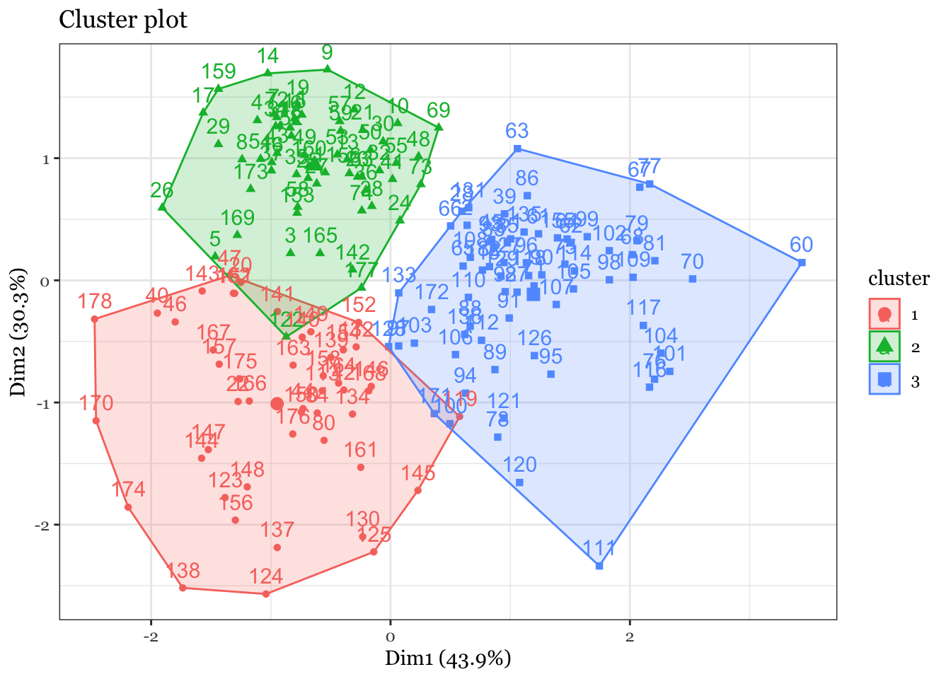
fviz_cluster(wine_cluster, data = wine_subset, ellipse.type = "norm") + 
  theme_bw() +
  theme(text = element_text(family="Georgia")) 

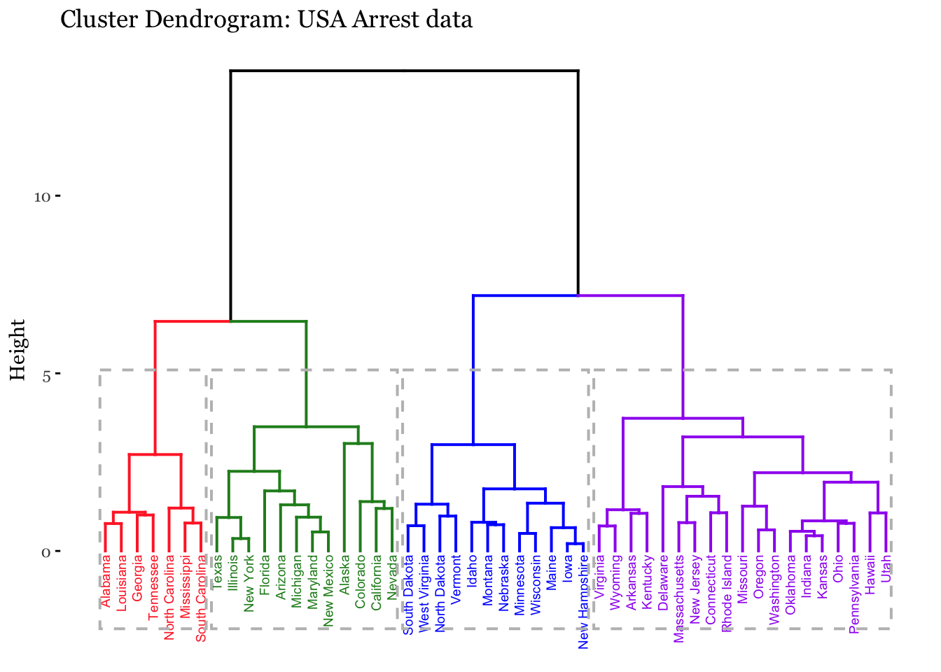
## Hierarchical Clustering
## Dataset: USArrests
#  install.packages("cluster")
arrest.hc <- USArrests %>%
  scale() %>%                    # Scale all variables
  dist(method = "euclidean") %>% # Euclidean distance for dissimilarity 
  hclust(method = "ward.D2")     # Compute hierarchical clustering

# Generate dendrogram using factoextra package
fviz_dend(arrest.hc, k = 4, # Four groups
          cex = 0.5, 
          k_colors = c("firebrick1","forestgreen","blue", "purple"),
          color_labels_by_k = TRUE, # color labels by groups
          rect = TRUE, # Add rectangle (cluster) around groups,
          main = "Cluster Dendrogram: USA Arrest data"
) + theme(text = element_text(family="Georgia")) 

Warning: The `<scale>` argument of `guides()` cannot be `FALSE`. Use "none" instead as
of ggplot2 3.3.4.
ℹ The deprecated feature was likely used in the factoextra package.
  Please report the issue at <https://github.com/kassambara/factoextra/issues>.