      Year           Lag1                Lag2                Lag3
 Min.   :2001   Min.   :-4.922000   Min.   :-4.922000   Min.   :-4.922000
 1st Qu.:2002   1st Qu.:-0.639500   1st Qu.:-0.639500   1st Qu.:-0.640000
 Median :2003   Median : 0.039000   Median : 0.039000   Median : 0.038500
 Mean   :2003   Mean   : 0.003834   Mean   : 0.003919   Mean   : 0.001716
 3rd Qu.:2004   3rd Qu.: 0.596750   3rd Qu.: 0.596750   3rd Qu.: 0.596750
 Max.   :2005   Max.   : 5.733000   Max.   : 5.733000   Max.   : 5.733000
      Lag4                Lag5              Volume           Today
 Min.   :-4.922000   Min.   :-4.92200   Min.   :0.3561   Min.   :-4.922000
 1st Qu.:-0.640000   1st Qu.:-0.64000   1st Qu.:1.2574   1st Qu.:-0.639500
 Median : 0.038500   Median : 0.03850   Median :1.4229   Median : 0.038500
 Mean   : 0.001636   Mean   : 0.00561   Mean   :1.4783   Mean   : 0.003138
 3rd Qu.: 0.596750   3rd Qu.: 0.59700   3rd Qu.:1.6417   3rd Qu.: 0.596750
 Max.   : 5.733000   Max.   : 5.73300   Max.   :3.1525   Max.   : 5.733000
 Direction
 Down:602
 Up  :648
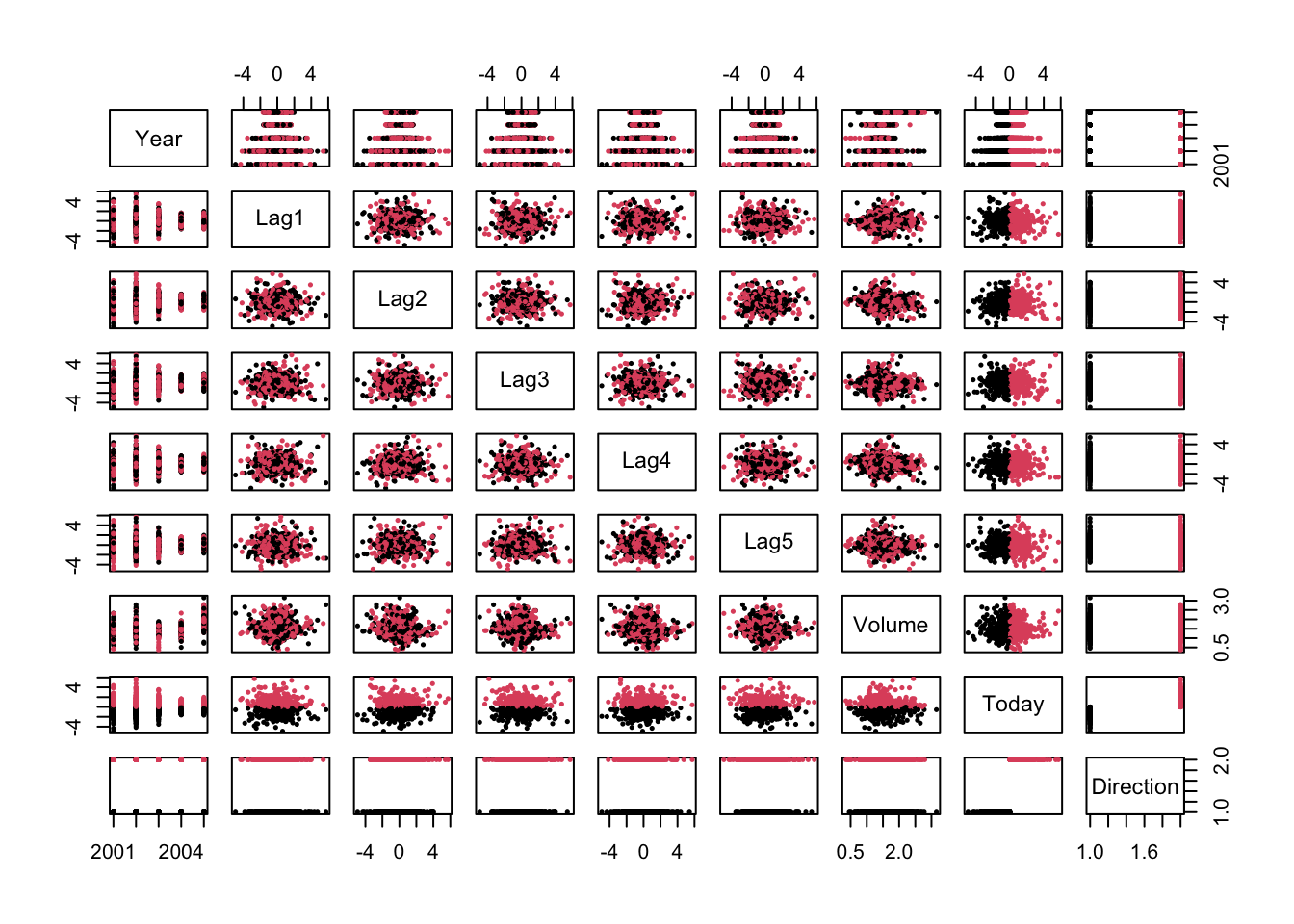
# Create a dataframe for data browsingsm=Smarket# Bivariate Plot of inter-lag correlationspairs(Smarket,col=Smarket$Direction,cex=.5, pch=20)
        Direction
glm.pred Down  Up
    Down  145 141
    Up    457 507
mean(glm.pred==Direction)
[1] 0.5216
# Make training and test set for predictiontrain = Year<2005glm.fit=glm(Direction~Lag1+Lag2+Lag3+Lag4+Lag5+Volume,data=Smarket,family=binomial, subset=train)glm.probs=predict(glm.fit,newdata=Smarket[!train,],type="response") glm.pred=ifelse(glm.probs >0.5,"Up","Down")Direction.2005=Smarket$Direction[!train]table(glm.pred,Direction.2005)
        Direction.2005
glm.pred Down Up
    Down   77 97
    Up     34 44
        Direction.2005
glm.pred Down  Up
    Down   35  35
    Up     76 106
mean(glm.pred==Direction.2005)
[1] 0.5595238
# Check accuracy rate106/(76+106)
[1] 0.5824176
# Interpretation:## The model correctly predicted the direction of the stock market 48% of the time ## when fitted to a set with all the variables## When fit to a smaller data set (some variables removed) the model predicts ## direction with 56% accuracy. This higher accuracy score suggests that lag1 and ## lag2 have a stronger relationship to the direction of the stock market## The model is has an accuracy score of 58% when predicting "up", which means## for some reason the model is better at predicting just "up" compared to both## up and down
Part 2
a. What is/are the requirement(s) of LDA?
predictor variables should follow a normal dist
observations should be independent to each other
linear relationship
Co-variance measurements are identical in each class
b. How LDA is different from Logistic Regression?
They are both binary classification methods for statistical analysis. There are many differences, here are a few:
-LDA assumes the predictors have a normal distribution whereas logistic regression makes no assumptions
-Logistic regression is based on maximum likelihood estimation, meaning it is trying to maximize the likelihood of observing the data given the parameters. LDA uses least squares estimation and is trying to maximize the separation between different classes.
-Logistic regression can handle more predictors compared to observation, LDA has issues with this because it assumes the predictors have a normal distribution
c. What is ROC?
Receiver Operating Characteristic. An ROC curve is a probability curve that is used to measure the performance of a binary classification model. In this graph, sensitivity is plotted on the Y-axis and specificity is plotted on the X-axis. This shows how specificity and sensitivity are graphed together, the area under the curve is what quantifies the performance of the model as a whole. If the area under the ROC curve is 1.
d. What is sensitivity and specificity? Which is more important in your opinion?
Sensitivity is the accuracy for the positive values and specificity the accuracy for the negative values.
In this case, sensitivity measures the TP … how accurate a “yes” was predicted as a “yes”. Sensitivity = TP / (TP + FN)
Specificity measures TN… how accurate the model predicted a “no” when it was a “no”
In my opinion It depends on the problem you’re trying to solve if specificity or sensitivity is more important. In a case where you are predicting a life threatening disease, sensitivity is more important because its okay to have more false positives than false negatives. In a situation like stock market where you are trying to maximize profit, sensitivity would be more important. If you are trying to minimize loss, specificity would be more important.
e. From the following chart, for the purpose of prediction, which is more critical?
TP and TN are the most critical for prediction because they tell you how often your prediction was right
3. Calculate the prediction error from the following …